
We've all been there: staring at a spreadsheet with hundreds, maybe thousands, of empty rows that need filling. It's daunting. But what if you could populate all that data with just a few clicks? That's exactly what autofill in Google Sheets is for. It’s less of a feature and more of a productivity powerhouse, designed to turn mind-numbing manual entry into a quick, automated process.
Think about creating a project timeline. You need to list out dates, sequential task numbers, or maybe even repeating employee assignments. Typing that out one by one is a guaranteed way to waste an afternoon and introduce a bunch of typos. This is where autofill shines. It's smart enough to spot patterns in your data and extend them for you, saving you a ton of hassle.
This guide will walk you through the whole spectrum of autofill techniques. We'll start with the basics, like the surprisingly powerful little blue fill handle, and work our way up to dynamic formulas that can populate entire columns automatically. My goal is to help you see your spreadsheets as a tool for automation, not just data storage.
Choosing the Right Autofill Strategy
Not all autofill tasks are created equal. The trick is knowing which tool to grab for the job at hand. Are you just filling a simple series of numbers or dates? The fill handle is your best friend. But if you're dealing with more complex logic or data that needs to update on its own, you'll want to lean on formulas like ARRAYFORMULA.
This flowchart gives you a good mental model for deciding which approach to take.
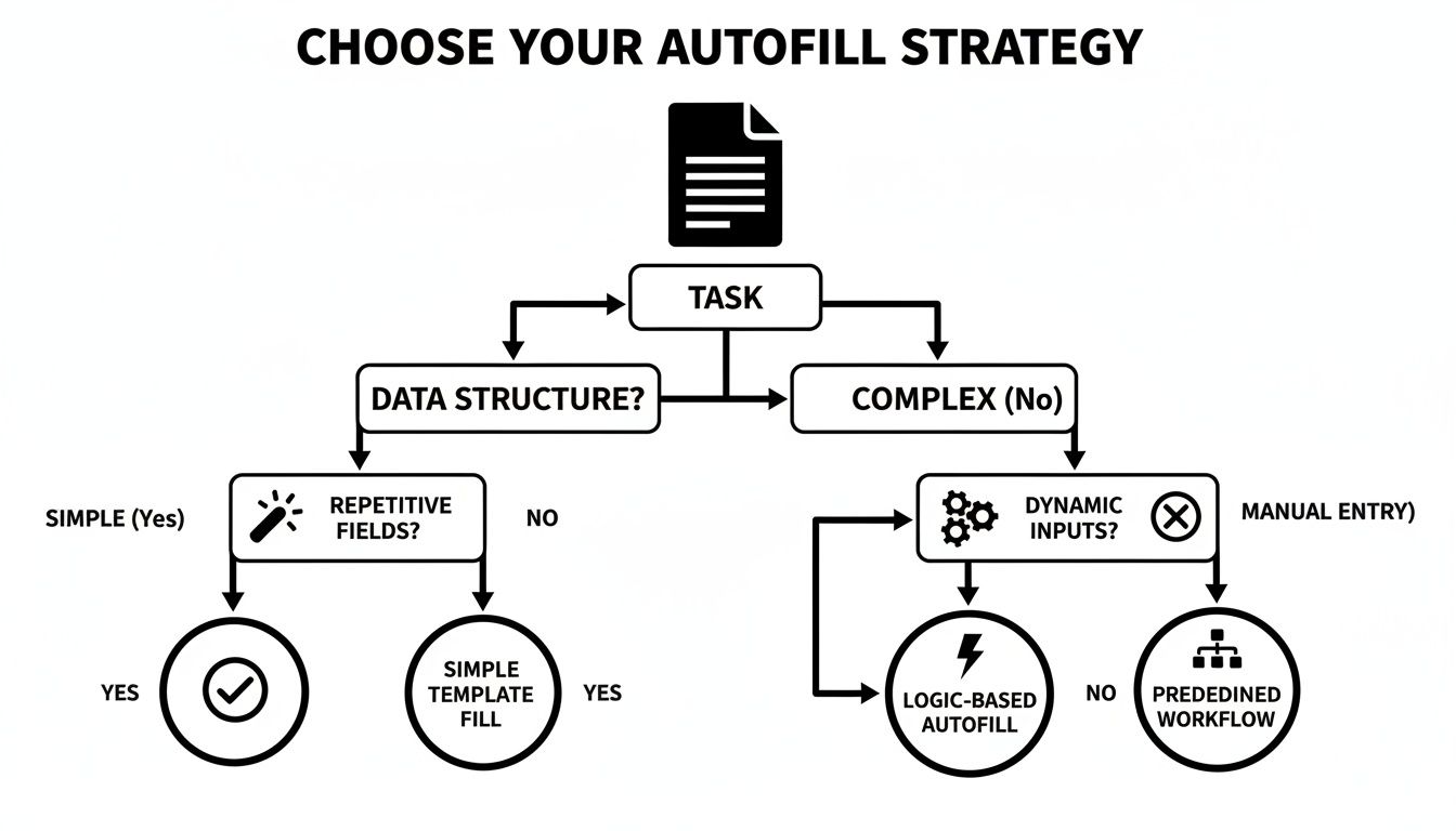
It really comes down to matching the tool to the task. Simple jobs call for simple tools; complex data structures benefit from the power and flexibility of formulas.
To help you get started, here's a quick overview of the essential autofill methods we'll be covering. Think of this as your go-to reference for picking the best technique for any situation.
Your Google Sheets Autofill Toolkit
A quick overview of the essential autofill methods we'll cover, helping you find the right tool for your specific data entry task.
| Technique | Best Use Case | How It Works |
|---|---|---|
| Fill Handle (Drag-Down) | Simple sequential data (numbers, dates, days) or copying a value/formula. | Click the small blue square on a cell and drag it down or across. |
| Fill Handle (Double-Click) | Quickly filling a column down to the last row of an adjacent column. | Double-click the fill handle instead of dragging it. |
| Custom Lists | Filling non-standard sequences (e.g., department names, project stages). | Create a custom list in settings, then use the fill handle to apply it. |
| Smart Fill | Automatically extracting or combining data from other columns (e.g., names from emails). | Start typing a pattern, and Google Sheets will suggest the rest. |
ARRAYFORMULA |
Applying one formula to an entire column, so it updates automatically with new rows. | Wrap your formula in ARRAYFORMULA() to apply it to a range instead of a single cell. |
Each of these methods has its place, and knowing when to use which one is what separates a casual user from a Sheets pro.
The impact here is huge. I’ve seen teams cut their data entry time by up to 80% on repetitive tasks just by mastering these techniques. It also dramatically improves accuracy—manual entry can introduce errors in as many as 5-10% of cells in large datasets. You can learn more about these productivity wins and find other time-savers by checking out our other Google Sheets tips.
At its core, autofill is about reclaiming your time. Every drag of the fill handle is a moment you're not spending on tedious, manual input, freeing you up to focus on analysis and strategy instead.
Getting to Know the Fill Handle
The heart of autofill in Google Sheets is a tiny but mighty feature called the fill handle. It’s that small blue square you see in the bottom-right corner of any cell you click on. It might not look like much, but this little handle is your key to cutting out tons of repetitive data entry.
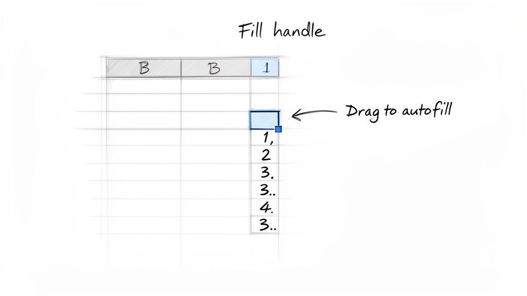
Let's say you're building a monthly sales tracker and need a column for every day of the month. Instead of typing out each date by hand, you just give Sheets a pattern to follow. Enter the first two dates, select both cells, then grab that fill handle and drag it down. Just like that, Sheets sees the daily pattern and populates the rest of the column for you. This works for all sorts of things—numbers, days of the week, or even text that follows a pattern.
Creating Simple and Complex Series
The fill handle is surprisingly smart; it can pick up on all kinds of sequences. You just have to give it a little nudge in the right direction.
- Sequential Numbers: Pop a
1in a cell and a2right below it. When you select both and drag, Sheets knows you want3, 4, 5...and continues the series. - Predictable Text: Type
Task 1into a cell. Drag the fill handle, and it will automatically generateTask 2,Task 3, and so on. This is a lifesaver for project plans or to-do lists. - Date Patterns: Need to list out weekly dates? Enter
1/1/2025in one cell and1/8/2025in the next. Sheets gets the hint and will fill in1/15/2025,1/22/2025, etc., when you drag.
This trick isn't just for values; it’s a formatting powerhouse, too. A neat feature that has improved a lot over the years is how autofill handles styles. If you select a cell with 'January' (bold) and the one below it has 'February' (italic), dragging the handle will continue the pattern, alternating between bold and italic for 'March', 'April', and beyond. You can create hundreds of styled entries instantly. For a deeper dive into these capabilities, check out this great resource on how Sheets recognizes patterns on Dataful.tech.
The Double-Click Shortcut for Large Datasets
Dragging the fill handle is perfect for a few dozen rows, but what if you have a dataset with thousands of entries? This is where a simple double-click becomes one of your best friends in Sheets. It's one of my go-to moves when I'm wrangling a lot of data.
Instead of dragging, just move your cursor over the fill handle until it turns into a crosshair and double-click.
This single action tells Google Sheets to fill the data all the way down to the last row of the adjacent column. It’s smart enough to stop exactly where the neighboring data ends, so you don't have to worry about going too far or not far enough.
I find this incredibly useful after pasting a big chunk of data into one column and needing to add an index number or a date series right next to it. What could have been a tedious drag-and-scroll marathon becomes a single, satisfying click. It’s a non-negotiable technique for anyone who wants to get serious about mastering autofill in Google Sheets.
Automating Calculations with Formulas
While filling in dates and numbers automatically is handy, the real magic of autofill in Google Sheets happens when you start using it with formulas. This is where your spreadsheet goes from being a static table to a dynamic calculator that does the heavy lifting for you.
Think about calculating sales commissions. You might write one formula to figure out the commission for the first salesperson. Instead of manually copying and pasting that formula for hundreds of others, a quick drag of the fill handle does it all instantly.
Relative vs. Absolute References: The Key to Smart Formulas
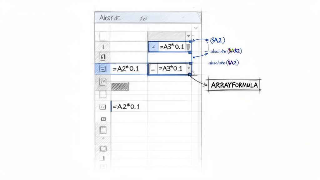
When you drag a formula down a column, Google Sheets is pretty clever. It automatically adjusts the cell references for you. This is the whole idea behind relative references. If your formula in cell C2 is =A2*B2, dragging it down to C3 intuitively changes it to =A3*B3.
But what happens when one part of your formula needs to stay put? Maybe you have a single commission rate in cell E1 that applies to every single sale. If you drag a normal formula, E1 will become E2, then E3, and everything will break. This is exactly why we have absolute references, marked with a dollar sign ($).
- Relative Reference (
A1): The default. Both the column and row change as you fill. - Absolute Reference (
$A$1): Completely locked. Neither the column nor the row will change, no matter where you drag the formula. - Mixed Reference (
$A1orA$1): A hybrid. You can lock just the column ($A) or just the row ($1), letting the other part adjust.
In our commission scenario, the formula would look like this: =A2 * $E$1. Now when you drag it down, A2 will correctly update to A3, A4, and so on, but $E$1 will always point back to that single commission rate cell.
The Superior Approach: Using ARRAYFORMULA
Dragging formulas is great, but it has a fundamental weakness: every single cell in your column has a separate, vulnerable formula. If a teammate accidentally types over a cell in the middle of your calculated column, that one calculation is broken. A much more bulletproof method is to use the ARRAYFORMULA function.
ARRAYFORMULA lets you place a single, powerful formula in one cell that populates an entire range with results. You only have one formula to edit, making your sheet cleaner and incredibly resistant to accidental changes.
The biggest win with
ARRAYFORMULAis resilience. The formula lives in just one cell (usually in the header), so users can't accidentally delete or overwrite the logic in individual rows. It protects your data integrity.
Let's walk through a real-world example. Say you want to check if sales values in column B (starting from B2) hit a target of $500. The old way would be to put =IF(B2>=500, "Met", "Not Met") in C2 and drag it down.
With ARRAYFORMULA, you put this in C1 instead:=ARRAYFORMULA(IF(B2:B="", "", IF(B2:B>=500, "Met", "Not Met")))
Let's break that down:
ARRAYFORMULA(...): This wrapper tells Google Sheets to apply the logic inside to an entire range, not just one cell.IF(B2:B="", "", ...): This is a pro-level trick. It first checks if a cell in theBcolumn is empty. If it is, it leaves the corresponding cell in your formula column blank, keeping your sheet tidy.IF(B2:B>=500, "Met", "Not Met"): This is your core logic, but now it operates on the entireB2:Brange at once.
With this single formula in place, your "Status" column will update automatically as new sales data comes in. For more ideas on how to chart this kind of data, you can learn to create a line of best fit in our detailed guide.
Using AI-Powered Smart Fill and Custom Lists
Beyond just filling in simple number sequences, the real magic of Google Sheets autofill is how it understands context and adapts to your specific needs. This is where AI-driven features and your own custom lists turn what used to be a tedious chore into a simple click-and-drag.
Let Smart Fill Do the Heavy Lifting
Ever find yourself with a column of full names, needing to quickly pull out just the first names? Or maybe you have address components—street, city, state—in separate columns that need to be merged into one. In the past, this meant wrestling with complex formulas. Not anymore.
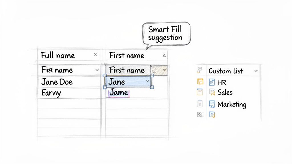
This is exactly what Smart Fill was built for. It’s a seriously smart feature that automatically detects patterns between your columns. You just have to show it what you want.
Start typing the desired outcome in a new, adjacent column. After you manually enter just one or two examples, Sheets will analyze what you're doing, figure out the pattern, and offer to complete the entire column for you in a flash.
For example, if you have "Jane Doe" in column A and you type "Jane" next to it in column B, Sheets will likely pop up a greyed-out suggestion box, ready to fill in "John" for "John Smith" in the next row, and so on down the line. Just click the checkmark, and your work is done.
Smart Fill is practical AI in action. It doesn't just fill a sequence; it deciphers your goal, saving you from the headache of writing
LEFT,RIGHT, andCONCATENATEformulas for everyday data wrangling.
Creating Custom Autofill Lists for Your Workflow
While Sheets is great with built-in lists like days of the week or months of the year, most businesses operate on their own unique cycles. Think about your specific project stages, regional office locations, or a recurring rotation of team duties. Typing these out over and over is a waste of time and an invitation for typos.
This is your chance to teach autofill in Google Sheets your own custom lists. Now, unlike Excel, Sheets doesn't have a dedicated menu to permanently save custom lists. But don't worry—the workaround is incredibly simple and effective.
Here’s how you can create a custom list on the fly:
- Define Your Sequence: In any column, type out your list items in the exact order you want them to appear. For example, you could type "Planning" in one cell, "Execution" in the next, and "Review" in the one below.
- Select the Pattern: Highlight the cells containing your complete sequence. In our example, you'd select the three cells with your project stages.
- Drag the Fill Handle: Click and drag the fill handle down the column. Google Sheets will perfectly repeat your custom sequence—Planning, Execution, Review—for as many cells as you need.
This trick is a lifesaver for standardizing data entry. By setting up a clear pattern for things like project statuses or department names, you ensure everyone on your team is using consistent terminology. It’s a simple but powerful way to make the autofill google sheets feature work for your specific processes, leading to cleaner, more reliable data.
Managing Autofill on Large Datasets
If you’ve ever tried to double-click the fill handle on a column with 50,000 rows, you’ve probably seen the dreaded "Page Unresponsive" error. It’s a frustrating but common wall that many of us hit when working with serious data. The problem is pretty straightforward: Google Sheets is a web app, and your browser only has so much memory to spare.
When you ask it to instantly create and calculate tens of thousands of new cells, you're maxing out your computer’s local resources. The browser tab freezes, sputters, and eventually gives up. This bottleneck can turn a simple task into a total dead end, especially when dealing with enterprise-level datasets.
Beyond Browser Limitations
The fix isn't a more powerful computer—it’s a different workflow. When your browser can't handle the processing, you need to shift that work to a server built for heavy lifting. That's exactly where professional tools come into play.
Instead of forcing your browser to do all the work, these services process massive CSV or Excel files on their own powerful backend servers. Once the data is ready, it's carefully streamed into your Google Sheet in a way that doesn't trigger a browser meltdown.
This server-side approach is a complete game-changer. It lets you work with hundreds of thousands or even millions of rows without ever seeing a crash.
The key takeaway is that for massive datasets, you must move the processing load from your local browser to a dedicated server. This is the only reliable way to bypass the inherent performance limits of web applications like Google Sheets.
Preserving Formulas During Large Imports
One of the biggest wins of using a dedicated import tool is how it protects the formulas you've already set up. Many of us have sheets with clever ARRAYFORMULA columns ready to process any new data that comes in. If you manually paste 100,000 new rows, you risk breaking or completely overwriting those essential formulas.
A smart import tool knows to append the new data without touching your existing headers and formula rows. It ensures that as soon as the new data lands, your formulas kick in and apply to every new entry, keeping your entire workflow automated and intact.
This approach bridges the gap between the everyday convenience of autofill in Google Sheets and the real-world demands of large-scale data. If this is a problem you're struggling with, our guide on how to upload large CSVs to Google Sheets without crashes dives deeper into the solution.
Got Questions About Autofill? Let's Solve Them.
Even the handiest tools have their quirks, and autofill is no exception. Sometimes it just doesn't cooperate, or you're trying to figure out how it handles a specific formula. It happens to everyone. Let's walk through some of the most common hangups I see people run into.
The classic problem is when autofill just... doesn't. You drag the little blue square and nothing happens, or it just copies the same value over and over. Nine times out of ten, it’s one of two things. First, make sure you're actually grabbing the fill handle—that tiny square—and not just the cell border. It's an easy mistake to make.
The other common culprit is not giving Sheets enough information to see a pattern. If you want a sequence like 1, 2, 3..., you have to select at least two cells with "1" and "2" in them. If you just select the cell with "1" and drag, Sheets thinks you just want to copy "1" everywhere. You have to establish the pattern first.
Why Isn't My Autofill Working?
Beyond those basic missteps, a few other things can trip you up. If you have hidden rows or an active filter, autofill will stop dead in its tracks when it hits them. It's a good habit to clear any filters before you try to fill a large range of cells.
And what about that magical double-click trick? It's a massive time-saver, but it has one very specific rule: it needs an adjacent column of data right next to it. Sheets uses that column to figure out where to stop filling. If you try it on a standalone column with nothing next to it, it won't know what to do.
Creating Your Own Custom Fill Lists
What if you need to repeat a custom sequence, like "High," "Medium," and "Low" for task priorities? While Sheets doesn't have a dedicated menu for saving these lists like Excel does, the on-the-fly method is incredibly simple.
- First, just type your list out in a few cells. Put "High" in A1, "Medium" in A2, and "Low" in A3.
- Next, select all three of those cells to show Sheets the complete pattern.
- Now, just drag the fill handle down. Sheets will repeat that exact sequence—High, Medium, Low—for as long as you drag.
For lists you use all the time, the best workaround is to create a "helper" tab in your workbook. Just keep your master lists there, and you can quickly copy-paste or reference them whenever you need them.
The real power of autofill shines when you understand how it handles formula references. It's smart enough to adjust relative references (like
A1) but keep absolute references ($A$1) locked in place. This is the secret to applying something like a single tax rate to thousands of rows without a single error.
Imagine a formula like =A1*B$1. When you drag that down, it becomes =A2*B$1 in the next cell. The A1 part correctly shifts to the next row, but the $B$1 stays put—perfect when you're multiplying everything by a constant value in cell B1. Getting comfortable with this is a game-changer for building reliable spreadsheets.
When your dataset gets too big, trying to autofill thousands of rows can bring your browser to a screeching halt. SmoothSheet was built to fix this. It offloads the heavy processing to powerful servers, so you can import millions of rows directly into Google Sheets without the lag, freezes, or crashes. Give it a try for free and see what a difference it makes. Learn more at SmoothSheet.