Google Sheets Linking to Another Sheet Made Easy

Let's face it, we've all been there: stuck in the copy-paste nightmare, bouncing between tabs and files just to keep our reports updated. It’s tedious, and worse, it’s a recipe for costly mistakes. This is where connecting your Google Sheets becomes a total game-changer.

Instead of manually moving data around, you can create a living, breathing system where information flows automatically. You can pull specific data from one sheet into another using simple formulas—like ='Sheet Name'!A1 for tabs in the same file or the powerful IMPORTRANGE function to connect completely separate spreadsheets.

Why Connecting Google Sheets Is a Game Changer

The real magic happens when you stop thinking of your spreadsheets as isolated documents and start treating them as an interconnected network. Linking your sheets lets you build dynamic dashboards and reports that update in real-time. This isn't just a minor convenience; it frees you from mind-numbing data entry so you can focus on what the numbers actually mean.

Create a Single Source of Truth

When you link your data, you establish a central hub for information that everyone can trust. Imagine a sales team where each regional manager's numbers automatically feed into a master dashboard, or a marketing team that pulls campaign results from multiple ad platform exports into one central ROI report. No more second-guessing if you have the latest version.

This approach delivers some serious benefits:

• Drastically Improved Accuracy: Linking eliminates the human errors that inevitably creep in with manual data entry.
• Huge Time Savings: Updates happen on their own, giving you back hours every week for more important work.
• Better Team Collaboration: Everyone works from the same playbook, with a clear, unified view of key metrics.

Boost Efficiency and Make Smarter Decisions

The shift to remote work really put a spotlight on how critical this is. We saw a massive spike in cross-sheet referencing back in early 2020 as teams scrambled to stay connected. One analysis I came across even found that finance teams saved an average of 12 hours a week just by using VLOOKUP to connect sheets for consolidation tasks. You can dig into similar findings over at Statology.

This is more than just a clever spreadsheet trick; it’s a fundamental shift in how you manage and interact with your data. By linking your sheets, you're building a reliable, scalable system that ensures your reports are always accurate and ready for action.

If you're someone who regularly pulls in large datasets from different places, linking becomes even more powerful when you pair it with the right tools. You can explore some of the best Google Sheets add-ons for data import to see how they can handle bigger, more complex workflows. Building this kind of connected ecosystem will save you countless hours and keep your data pristine.

Using IMPORTRANGE to Connect Different Workbooks

When you need to pull data from a completely separate Google Sheets file, IMPORTRANGE is the function you'll reach for. Think of it as the big brother to the simple cell references we used earlier. While those work great inside a single workbook, IMPORTRANGE builds a live bridge between two different files.

This is a game-changer for consolidating information. I use it constantly to pull sales figures from regional reports into a master dashboard or grab project updates from various team sheets to see a high-level overview. It completely removes the need to manually copy and paste data—a process that’s not just tedious but also a huge source of human error.

This flow diagram really captures the essence of how linking sheets turns raw, scattered data into a clean, actionable dashboard.

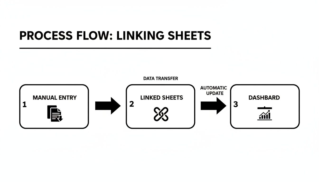
The real magic here is how a simple function acts as the glue, holding together an automated reporting system.

Understanding the IMPORTRANGE Syntax

At its core, the function is surprisingly simple. It just needs two pieces of information: the URL of the Google Sheet you want to pull from and the specific cells you want to grab.

The formula looks like this: =IMPORTRANGE("spreadsheet_url", "sheet_name!range_string")

Let's break that down:

• spreadsheet_url: This is the full web address of the source Google Sheet. Just copy it from your browser's address bar and make sure to wrap it in double quotes.
• sheet_name!range_string: This tells Google Sheets exactly which tab and cells to import. For instance, "Q4 Sales!A2:F50" would pull columns A through F from a tab named "Q4 Sales."

This function really became a workhorse for business analysts around 2018 when Google Sheets started getting serious adoption. I remember reading studies back then estimating it cut down manual data entry by as much as 40% for some finance teams.

Handling the #REF Error and Granting Access

The very first time you use IMPORTRANGE to connect to a new spreadsheet, you're going to see a #REF! error. Don't worry—this is completely normal. It’s Google’s way of asking for your permission before it lets two separate files start sharing data.

Fixing it is easy. Just hover your mouse over the cell with the error, and a blue button will pop up with the message "Allow access." Click it, and your data will appear instantly. This is a one-time security check for that specific connection; you won't have to do it again for that link.

Making Your Links More Resilient with Named Ranges

Here’s a pro tip. One of the biggest headaches with IMPORTRANGE is when the formula breaks because someone adds a row or column to the source sheet, shifting your data range. The best way to avoid this is by using Named Ranges.

A Named Range is basically a friendly, fixed name (like "Q1_Sales_Data") that you assign to a range of cells (like 'Sales'!A2:G). The beauty is, if you add new rows within that range, the Named Range automatically expands to include them.

So, instead of a fragile reference like 'Sales'!A2:G50, you can create a Named Range called SalesData in your source file. Your formula then becomes much cleaner and more robust:

=IMPORTRANGE("spreadsheet_url", "SalesData")

This simple trick makes your formulas far more durable. They’ll keep working correctly even as the source data grows and changes over time. If you want to dive deeper, check out our complete guide to mastering the IMPORTRANGE function.

Linking Between Tabs in the Same Spreadsheet

While IMPORTRANGE is your go-to for pulling data between separate workbooks, what about linking different tabs, or sheets, within the same file? This is a much more common task, and thankfully, the solution is a lot simpler. It’s called direct sheet referencing, and it's the bread and butter of organizing data inside a single spreadsheet.

I use this all the time for creating summary dashboards. Just imagine you have separate tabs for each month's sales—"Jan Sales," "Feb Sales," and so on. You can easily build a "Q1 Summary" tab that pulls the grand total from each of those monthly sheets, giving you a clean, at-a-glance overview.

Mastering the Basic Syntax

The syntax for linking to another sheet is elegantly simple. You just need the sheet name, an exclamation mark, and the cell you want to pull from.

The basic formula looks like this: ='Sheet Name'!CellReference

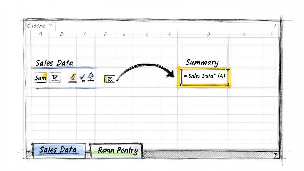
So, if you wanted to pull the value from cell A1 in a sheet named "Sales Data," you'd just type ='Sales Data'!A1 into a cell on another tab. That’s it. No permission pop-ups, no long URLs to copy. It just works.

Here's a pro-tip: If your sheet name has spaces or special characters (like "Sales Data" or "Q1-Report"), you absolutely must wrap the name in single quotes. If the name is just one word, like "Sales," the quotes are optional, but I find it's a good habit to use them anyway to avoid errors down the road.

And this isn't just for pulling a single cell. You can use this syntax inside almost any function that needs a range.

Building Dynamic Dashboards with Formulas

The real magic of direct referencing happens when you start combining it with other functions. This is how you can aggregate, calculate, and summarize data from across your entire workbook onto a single, powerful dashboard.

Here are a few ways I use it all the time:

• Summarizing Totals: Need the sum of all sales from your "Jan Sales" tab? Just use =SUM('Jan Sales'!F:F).
• Counting Entries: Want to know how many clients are on your "Client List" tab? A formula like =COUNTA('Client List'!A2:A) will do the trick.
• Creating Lookups: You can even run a VLOOKUP that searches for a value on one sheet and pulls its matching data from a master list on another tab.

This method is incredibly efficient for keeping your workbook organized. It lets you keep related data together in one file while still allowing for clean, compartmentalized reporting.

But be aware of one major vulnerability. If you rename the source sheet, Google Sheets is pretty smart and will usually update your formulas automatically. However, if you move the source data by cutting and pasting cells, your references can easily break, leaving you with a bunch of frustrating #REF! errors. Because of this, it's best for workbooks where the data structure is relatively stable.

Solving Common Linking Errors and Issues

Even the most experienced Google Sheets pros run into trouble now and then. When you start linking sheets, especially with IMPORTRANGE, you're bound to hit a few error messages. But don't worry—most of these are surprisingly easy to fix once you know what to look for.

The most common issue you'll face is the dreaded #REF! error. It almost always pops up for one of two reasons: you either haven't granted permission for the two sheets to connect, or there’s a tiny syntax mistake in your formula. Before you do anything else, double-check that you've clicked the "Allow access" button and that your sheet names and cell ranges are spelled perfectly.

You might also see that persistent "Loading..." message. This is usually a sign that the source sheet is massive or your formula is a bit too complex, causing a calculation timeout. Sometimes, waiting a bit helps, but more often, it's a signal to find a more efficient way to pull your data.

Troubleshooting Common Formula Problems

Let's dig into the specific errors that can stop your workflow in its tracks when google sheets linking to another sheet goes wrong. These are the usual suspects, but they all have straightforward solutions.

A classic mistake is a simple typo in the URL or the range string. Seriously, a single incorrect character will break the entire formula.

• #REF! (Permission Error): This is the first thing you'll see with a new IMPORTRANGE. Just hover over the cell and click the blue "Allow access" button. Problem solved.
• #REF! (Syntax Error): Check your sheet name or range for typos. Remember, "Sales Q1!A:F" is completely different from "Sales-Q1!A:F". Precision is everything here.
• #N/A (Not Found): This error usually appears when you’ve wrapped IMPORTRANGE inside a lookup function like VLOOKUP, and the item you're looking for just isn't in the imported data.
• #VALUE! (Wrong Data Type): This often points to a formatting mismatch. A common scenario is trying to do math on a column that contains text, even if it looks like numbers.

If you’re still scratching your head, our detailed guide on how to fix common IMPORTRANGE errors has even more troubleshooting steps to get you back on track.

Optimizing Performance with Advanced Functions

Once you've got the basics down, you can seriously speed things up by nesting IMPORTRANGE inside other functions. This clever trick lets you filter and process data before it even arrives in your destination sheet, which drastically reduces the calculation load. The QUERY function is your best friend for this.

Imagine you need to import sales data for orders over $100 from a huge sales log. Instead of pulling in thousands of rows and then filtering them, you can do it all in one go:

=QUERY(IMPORTRANGE("spreadsheet_url", "SalesLog!A:G"), "SELECT Col1, Col2, Col7 WHERE Col7 > 100")

This formula tells Google Sheets to only grab columns 1, 2, and 7 for rows where the value in column 7 is greater than 100. It's so much faster and more efficient than importing a mountain of data you don't need.

This technique is a complete game-changer for building responsive dashboards. By pre-filtering your data, you keep your sheets lean and prevent them from getting bogged down.

Understanding Permission Settings

Permissions are a constant source of confusion, so let's clear things up. The access level on the source sheet is what determines if your link will work. For an IMPORTRANGE formula to succeed, the person who created it must have at least "Viewer" access to the source file.

Here's how access levels affect your links:

• Viewer Access: You can import the data perfectly, but you can't change anything in the source sheet.
• Commenter Access: Same as Viewer; you can pull the data without any issues.
• Editor Access: You can both import the data and, if you open the source file, make changes to it.

Here’s the important part: if someone without access to the source sheet opens your destination file, they'll just see a #REF! error. The data won't load for them because they don't have permission to see it. This is a critical security feature, ensuring that sensitive information isn't accidentally shared with the wrong people.

Managing Large Datasets Without Crashing Your Sheet

Linking data is a fantastic feature, but it can quickly turn into a performance nightmare. If you've ever tried using IMPORTRANGE with a source sheet that has tens of thousands of rows, you know the pain of that endless "Loading..." message. The browser freezes, the sheet becomes unresponsive, and you're left staring at a spinning wheel.

This happens because Google Sheets has its limits. When you pull massive amounts of data, your browser is doing all the heavy lifting. Every time the source data changes, your destination sheet has to re-calculate everything, which can easily overwhelm its resources. It's a recipe for frustrating calculation timeouts and sluggish dashboards.

Smart Optimization Tips for Better Performance

Thankfully, you're not helpless here. You can take a few smart steps to keep your linked sheets running smoothly, even when the data starts piling up. The trick is to be intentional about what you import. Don’t just grab everything and hope for the best—be surgical.

One of the single most effective changes you can make is to stop importing entire columns. Instead of pulling in columns that might have hundreds of thousands of empty cells, get specific.

• Define Your Columns: Instead of Sales!A:Z, use Sales!A1:F. This simple tweak tells Google Sheets to stop looking for data past column F, which dramatically cuts down the processing load.
• Cap Your Rows: If you only need the first 1,000 rows for your report, define that range explicitly: Sales!A1:F1000. This is far more efficient than pulling in everything.
• Filter First with QUERY: As we talked about earlier, wrapping your IMPORTRANGE inside a QUERY function is a game-changer. It filters the data before it ever hits your sheet.

The guiding principle here is simple: only import what you absolutely need. Every extra cell you pull in adds to the computational burden and slows your entire workbook down. Be ruthless about trimming your import ranges.

When Your Data Is Just Too Big

Sometimes, no amount of optimization is enough. When you're dealing with truly massive files—like a multi-million row CSV export from your CRM or an ad platform—your browser will probably crash before the data even finishes loading. This is where you need to look beyond the browser.

Server-side tools are built for this exact problem. They handle the heavy lifting of importing and parsing huge files on a powerful server, bypassing your browser's limitations entirely. You can upload a giant file, and the tool processes it in the background, feeding the clean, ready-to-use data into your Google Sheet.

This approach completely changes the game for scalability. Your dashboards, all connected via IMPORTRANGE, will just keep working. Millions of new rows can be added to the source sheet, and your reports will update without those crippling performance bottlenecks. If you find yourself constantly battling massive files, checking out a guide on how to import CSV to Google Sheets using these methods can save you a ton of frustration and keep your reports lightning-fast.

Questions That Always Come Up When Linking Sheets

Once you start pulling data between sheets, a few questions inevitably pop up. I've seen these trip up beginners and experienced users alike, so let's get you some quick answers to save you a headache down the road.

How Often Does IMPORTRANGE Actually Update?

This is probably the number one question people ask. The short answer is: it's automatic. When you change something in the source sheet, IMPORTRANGE should reflect that change in the destination sheet.

Usually, this happens within seconds. However, if you're working with massive datasets or have a ton of complex formulas, you might notice a lag of a few minutes. It just takes Google a moment to process everything.

If you can't wait and need to see the update right now, here’s a simple trick: just edit the formula. Click into the cell, add a space at the end, and then delete it. Hitting enter forces Google Sheets to go fetch the data again. A good old-fashioned browser refresh works wonders, too.

What Else Causes That Annoying #REF Error?

Ah, the dreaded #REF! error. After you've granted permission for the sheets to connect, this error is almost always due to a simple typo. When you find your google sheets linking to another sheet isn't working, the very first thing to do is check your syntax with a fine-tooth comb.

I can't tell you how many times I've seen a link break because of one tiny mistake. The two biggest culprits are a typo in the spreadsheet URL or a misspelled sheet name. Remember, the formula sees 'Q1 Sales' and 'Q1-Sales' as completely different things. Even an accidental extra space will break it.

Can I Link to an Old Version of a Google Sheet?

That’s a smart question, but unfortunately, the answer is no. Whether you're using IMPORTRANGE or a simple reference to another tab, you're always pulling from the live, most current version of that sheet. Google Sheets doesn't have a feature to link to a specific point in a file's version history.

If you need to lock in and reference a dataset from a particular moment, the best workaround is to create a snapshot. Just go to File > Make a copy. This gives you a static version of the sheet that you can link to without worrying about future changes.

By the way, if you're wrestling with massive datasets that are slowing your IMPORTRANGE functions to a crawl, SmoothSheet is built for that. It lets you import huge CSV or Excel files directly into Google Sheets without freezing your browser, and it keeps all your formulas and connections intact. You can learn more and get started for free.