How to Find Duplicates in Google Sheets: how to find duplicates in google sheets

Finding duplicates in Google Sheets is simpler than you might think. For a quick fix, you can use the built-in Data > Data cleanup > Remove duplicates tool to get rid of them for good. If you'd rather just see where they are, a custom formula like =COUNTIF($A:$A, A1)>1 paired with Conditional Formatting will make them pop right off the page.

Why Duplicate Data Is Silently Harming Your Spreadsheets

Before we dive into the step-by-step methods, it's crucial to understand why this matters. Duplicate data isn't just a minor spreadsheet annoyance; it's a silent saboteur that can seriously compromise your work. Think of it like a small crack in a foundation—it seems harmless at first, but over time, it undermines the integrity of every decision you make based on that data.

These unwanted entries sneak into your sheets in all sorts of ways. It could be a simple copy-paste mistake, a customer accidentally submitting a form twice, or a messy data import from two different systems. Whatever the cause, the consequences are always a headache.

The Real-World Impact of Bad Data

Duplicate records create a ripple effect of chaos that can be surprisingly costly. A marketing team might spam the same customer with a promotion, leading to frustration and a quick unsubscribe. In finance, duplicate invoices could lead to accidental overpayments, hitting your cash flow directly. Imagine an inventory sheet with repeated product IDs—you might end up ordering too much stock or, worse, telling a customer something is available when it's long gone.

These aren't just hypotheticals. Poor data hygiene has tangible costs:

• Skewed Analytics: Your charts and reports will show inflated numbers, leading to flawed business strategies built on a house of cards.
• Wasted Time: Teams burn valuable hours manually cleaning up messes or dealing with the fallout from bad information.
• Damaged Customer Relationships: Redundant communications or incorrect records make your business look unprofessional and disorganized.

The Unreliability of Manual Checks

Trying to spot duplicates by just scanning your sheet with your eyes is a recipe for disaster. The human eye simply isn't built to find subtle patterns in large datasets, especially when the duplicates aren't sitting right next to each other.

This isn't just a feeling; it's a fact. Manual checks are incredibly unreliable. Research from the University of Michigan in 2023 found that people miss about 23% of duplicate entries when scanning datasets with more than 100 rows—even when they are actively looking for them. That's a huge margin of error. You can learn more about the challenges of manual data cleaning and see how automated tools can help.

Once you see the high stakes, finding and removing duplicates stops being a chore and becomes an essential business practice. Clean data is the bedrock of reliable analysis and smart decision-making.

See Your Duplicates at a Glance with Conditional Formatting

Sometimes, the best way to get a handle on a messy dataset is to actually see the problem. Before you start writing complex formulas or deleting rows, a quick visual check can tell you everything you need to know about the scale of your duplicate issue. This is where Google Sheets' Conditional Formatting really shines, turning a wall of text into a colorful map of redundant entries.

Instead of just highlighting a single duplicate cell, the real power comes from highlighting the entire row whenever a specific value is repeated. This gives you crucial context. Think about it: in a customer list, you don't just want to see a duplicate email address flagged; you want to see the whole record tied to it.

This simple visual cue helps you instantly understand what you're up against. Is it just a one-off copy-paste error, or do you have a bigger, systemic problem with how your data is being collected?

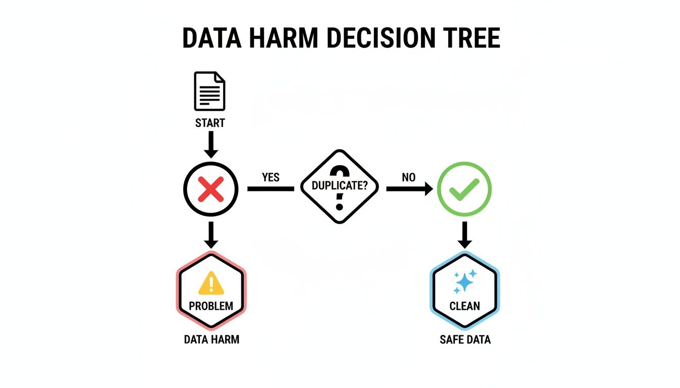
The flowchart above really simplifies the decision-making process. Once a duplicate is identified, it’s a data problem that needs attention. The key takeaway here is that duplicates aren't just harmless clutter; they actively degrade your data's quality and demand a clear, immediate response.

How to Set Up Your First Highlighting Rule

Let's walk through a classic scenario. You’ve just exported a list of leads from your CRM, and you need to flag any customer who shows up more than once. We'll use their email address in Column C as the unique identifier.

Here’s how you do it:

• First, select the entire range of your data. A quick way is to click the first cell of your data (say, A2, if you have headers) and drag down to the bottom-right cell.
• From the top menu, go to Format > Conditional formatting. This will pop open a sidebar where you'll create the rule.
• In the "Format rules" section, find the dropdown menu and select Custom formula is. This is where the magic happens.
• Now, in the formula box, you'll enter a special COUNTIF formula. This tells Google Sheets to count how many times each value appears in a specific column.

For our example, where emails are in Column C and our data runs from row 2 to 1000, the formula is: =COUNTIF($C$2:$C$1000, $C2)>1

Let’s quickly break down that formula so you know what it’s doing:

• $C$2:$C$1000: This is the absolute range where the formula will search for duplicates. The dollar signs $ are crucial—they lock the range so that every single row is checked against the entire column.
• $C2: This is the specific cell being checked. We lock the column ($C) but leave the row number (2) relative. As Sheets applies the rule down your selection, it will automatically check C3, C4, C5, and so on.
• >1: This is the trigger. If the count for any email is greater than one, the formatting rule kicks in.

Finally, pick a formatting style—a light red or yellow background fill usually works great for visibility. Click Done, and watch as every row with a duplicate email instantly lights up.

Practical Tips for Managing Your Rules

Once you get the hang of this, you might end up with several formatting rules. A little organization goes a long way. For instance, you could create one rule to highlight duplicate emails in yellow and a second rule to highlight duplicate order IDs in blue.

A quick heads-up: the order of your conditional formatting rules matters. Google Sheets applies them from the top down. If a cell meets the criteria for two different rules, the one that’s higher on the list gets applied.

Also, a word on performance. If you're working with a massive dataset (I’m talking 50,000+ rows), conditional formatting might cause a tiny bit of lag. Even so, running a highlighting rule is still one of the fastest ways to get a visual audit before you move on to deleting data.

Once you've seen your duplicates, the next logical step is to get your data organized. To explore different ways to do that, check out our handy guide on how to sort in Google Sheets.

Isolate and Analyze Duplicates with Formulas

Highlighting duplicates is a great way to see where the problems are, but it's a passive approach. You can see the issues, but you can't easily work with them. To really dig in, you need to pull those repeated entries into a separate, dedicated list.

This is where formulas come in. They let you extract, count, and analyze duplicate data with pinpoint accuracy, moving you from just spotting duplicates to actively managing them.

Imagine you have a sales log with thousands of entries. You don't just want to see which customers bought something more than once; you want a clean list of only those repeat customers to send a special "thank you" offer. Formulas make that happen.

We'll walk through two of the best methods: a flexible combination of FILTER and COUNTIF, and the incredibly powerful QUERY function. Both get you to a similar place but offer different levels of control.

Using FILTER and COUNTIF to List Duplicates

One of the most intuitive ways to create a list of just your duplicate values is by pairing the FILTER and COUNTIF functions. Here’s the simple logic: COUNTIF figures out which items show up more than once, and FILTER uses that information to build a new list containing only those items.

Let's say you have a list of product SKUs in Column A, from A2 to A100. You want a list of any SKU that appears multiple times.

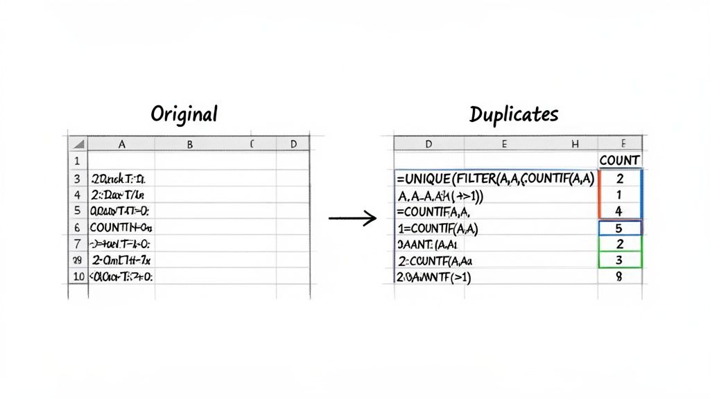
Find an empty cell and pop this formula in: =UNIQUE(FILTER(A2:A100, COUNTIF(A2:A100, A2:A100)>1))

I know that looks like a monster, but it's really just three simple steps happening at once:

1. COUNTIF(A2:A100, A2:A100)>1: This is the engine. It checks every single cell in the range A2:A100 against the entire list and flags it as TRUE if its count is greater than one (meaning it's a duplicate).
2. FILTER(A2:A100, ...): The FILTER function takes your original list and only keeps the rows where the COUNTIF check came back TRUE. The result is a list showing every single instance of a duplicate value.
3. UNIQUE(...): Finally, we wrap the whole thing in UNIQUE to clean up the output. Without it, the FILTER would return all occurrences (e.g., "SKU-123," "SKU-123," "SKU-123"). UNIQUE tidies this up, giving you a clean list with just one entry for each duplicated SKU.

This formulaic approach is non-destructive. Your original data remains untouched, giving you a safe space to analyze the duplicates without risk. This is a core principle of good data management—always preserve your raw data.

If you're looking to really master this, learning more about the FILTER function in Google Sheets is a great next step. Its flexibility is incredible when combined with other formulas.

Unleashing the Power of QUERY

If you're comfortable with a bit more structure, the QUERY function is a more robust and scalable way to find and count duplicates. It uses a syntax similar to SQL, letting you perform database-like operations right inside your sheet.

QUERY is especially handy when you want to not only list the duplicates but also see exactly how many times each one appears.

Using the same SKU list in A2:A100, you could start with this formula: =QUERY(A2:A100, "SELECT A, COUNT(A) GROUP BY A LABEL COUNT(A) 'Frequency'")

This instantly generates a two-column table. The first column lists every unique SKU, and the second, which we've named "Frequency," shows how many times it appeared.

To isolate just the duplicates, we just add a HAVING clause: =QUERY(A2:A100, "SELECT A, COUNT(A) WHERE A IS NOT NULL GROUP BY A HAVING COUNT(A) > 1 LABEL COUNT(A) 'Occurrences'")

Let's quickly decode what that statement is doing:

• SELECT A, COUNT(A): Tells the query to show the values from Column A and also count them.
• WHERE A IS NOT NULL: A good habit to get into. It stops the formula from counting blank cells.
• GROUP BY A: This is key. It lumps all identical values together so the COUNT function can work on them as a group.
• HAVING COUNT(A) > 1: This is the magic filter. It tells the query to only show groups that have a count greater than one—in other words, your duplicates.
• LABEL COUNT(A) 'Occurrences': This just renames the count column's header to something more readable.

The QUERY method is incredibly efficient, especially on larger datasets where nested FILTER and COUNTIF formulas might start to lag. It’s a clean, powerful way to find duplicates and a must-learn for anyone serious about spreadsheet analysis.

Alright, you've found the duplicates. Now what? Getting rid of them is the final step, but how you do it matters. You could permanently delete them with Google's built-in tool, or you could generate a fresh, clean list with a formula—a much safer, non-destructive approach.

The right method really depends on your goal. Are you just doing a one-time cleanup for a report, or do you need a live list that updates as new data comes in? Let's walk through both strategies so you can pick the best one for your situation.

Using the Built-In Remove Duplicates Tool

The quickest way to get rid of duplicate rows for good is with Google’s own cleanup tool. It's direct, powerful, and perfect for when you're absolutely sure you want those extra rows gone.

But first, a word of caution. Make a backup. Seriously. Just go to File > Make a copy. It takes two seconds and can save you from a world of hurt. This action is permanent—once those rows are deleted, you can't get them back.

With your copy safely tucked away, here's how to do it:

• Click any cell inside your data.
• Go to the menu and select Data > Data cleanup > Remove duplicates.
• A new window will pop up with some options.

In this menu, you'll see every column in your dataset. This is where you tell Sheets what counts as a "duplicate." For instance, if a customer's email in Column B is the unique thing you care about, you'd only check the box for Column B. Sheets will then zap every row with a repeated email, keeping only the first one it finds.

Pro Tip: Make sure the "Data has header row" box is checked if your sheet has headers. If you forget, Sheets might mistake your first row of data for a header, or worse, delete your actual header if it happens to match another row.

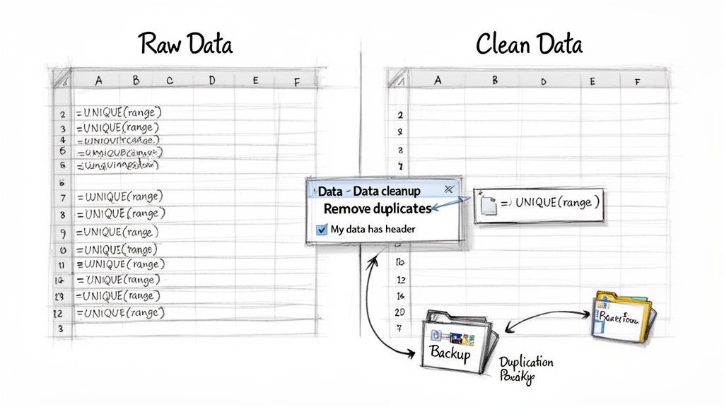
The Safer Alternative: The UNIQUE Formula

In many cases, permanent deletion is just too risky. What if you need to go back and check the original, messy data? A much safer and more flexible way to handle this is by using the UNIQUE formula. This lets you generate a brand-new, clean list somewhere else in your spreadsheet.

This method leaves your original data completely untouched, which is just good practice. It gives you a pristine list to work from while keeping the raw data safe for auditing or future analysis.

Just find an empty spot in your sheet (or on a new tab) and type this formula: =UNIQUE(A2:D1000)

You’ll want to replace A2:D1000 with the actual range of your data. The formula instantly spits out a new table containing only the unique rows from your source. Here, a "unique row" is one where the entire combination of values across all columns isn't repeated.

The best part? It's dynamic. If a new, unique row gets added to your original data, it automatically shows up in your UNIQUE list. No manual updates needed.

So, choosing between the two methods really comes down to one question: do you need to keep your original data? The built-in tool is great for quick, permanent cleanups, but the UNIQUE formula offers a safer, more flexible solution for ongoing projects. And if you're dealing with massive files that make Google Sheets choke, consider using an external CSV duplicate remover to clean the data before you even import it.

Going Beyond the Basics: Advanced Duplicate-Hunting Techniques

Simple duplicate checks are great, but real-world data is rarely so clean. You’ll inevitably run into messy situations—duplicates hiding behind different capitalization, entries scattered across multiple tabs, or datasets so big they make Google Sheets cry.

When the standard tools just can't keep up, you need to pull out the heavy artillery. Let's dive into some more powerful, nuanced ways to handle these complex problems and even automate the whole cleanup process for good.

How to Handle Case-Sensitive Duplicates

One of the most common headaches is case sensitivity. To Google Sheets, "[email protected]" and "[email protected]" are often treated as the same thing by default functions. But to a database or an email marketing platform, they could be two entirely separate records. This tiny detail can cause big data integrity problems down the line.

The fix is surprisingly simple: force everything into the same case before you check for duplicates. The LOWER() function is your best friend here. By wrapping your data range in LOWER(), you create a level playing field where "Apple" and "apple" are seen as true duplicates.

Here’s how you’d build this into a conditional formatting rule:

=COUNTIF(ARRAYFORMULA(LOWER($A$2:$A)), LOWER(A2))>1

Let's quickly unpack that formula:

• LOWER($A$2:$A) converts the entire column A to lowercase for the comparison.
• ARRAYFORMULA is the magic that makes LOWER() apply to the whole range at once, not just a single cell.
• LOWER(A2) converts the specific cell you're checking to lowercase.

This little tweak ensures you're doing a true apples-to-apples comparison, catching sneaky duplicates that would otherwise fly under the radar.

Automate Your Cleanup with Google Apps Script

If you find yourself cleaning the same sheet every week, it's time to stop doing it manually. Manual work is tedious and, frankly, prone to mistakes. This is where Google Apps Script comes in, letting you write your own little programs to automate just about anything in Sheets.

You can write a script to find and zap duplicates across your entire workbook—either with a single click or even on a schedule, like every Monday morning. Even if you’ve never touched code before, you can often adapt a basic script for your own needs.

Here's a simple script that removes duplicate rows based on the value in the first column of whatever sheet is currently active:

function removeDuplicateRows() { const sheet = SpreadsheetApp.getActiveSpreadsheet().getActiveSheet(); const data = sheet.getDataRange().getValues(); const uniqueData = {}; const rowsToDelete = [];

// Start from the end to avoid shifting row indices for (let i = data.length - 1; i >= 0; i--) { // Assumes the unique identifier is in the first column (index 0) const key = data[i][0]; if (uniqueData[key]) { rowsToDelete.push(i + 1); } else { uniqueData[key] = true; } }

// Delete rows in reverse order rowsToDelete.forEach(rowNum => { sheet.deleteRow(rowNum); }); }

To get this working, just go to Extensions > Apps Script, paste this code into the editor, save it, and click the "Run" button. This example looks at column A (data[i][0]), but you can easily change that to check a different column.

Keeping Your Sheet Fast with Large Datasets

Working with 50,000 rows or more changes the game entirely. The clever ARRAYFORMULA or QUERY functions that were instant on smaller sheets can suddenly become incredibly slow, making your browser lag or even crash.

When your sheet grinds to a halt, the problem usually isn't the formula itself. It's how many times that formula has to recalculate. Every single edit you make can trigger a massive chain reaction, forcing thousands of cells to update at once.

To get your sheet's performance back under control, here are a couple of my go-to strategies:

• Use Helper Columns: This is a big one. Instead of embedding a heavy formula directly into a conditional formatting rule, offload the work to a dedicated helper column. For example, in an empty column, just use the simple formula =COUNTIF($A$2:$A, A2)>1. This calculates the duplicate check once per row. Then, your conditional formatting rule becomes lightning-fast—it just has to check if the helper column says TRUE.

• Avoid Volatile Functions: Functions like NOW(), TODAY(), and RAND() are called "volatile" for a reason. They recalculate every time any change is made anywhere on the sheet, whether it's related or not. Keep them out of your large-scale duplicate checks to avoid unnecessary performance hits.

Thinking strategically about how your formulas run is the secret to managing how to find duplicates in Google Sheets at scale without pulling your hair out. It keeps your sheet snappy and responsive, no matter how much data you throw at it.

Dealing with Large Files Before You Can Find Duplicates

Sometimes, the biggest headache in finding duplicates isn't the formula—it's just getting your data into Google Sheets in the first place.

If you've ever tried to import a massive CSV or Excel file, you know the pain. The browser freezes, you get the "Page Unresponsive" error, and everything grinds to a halt. This isn't a Google Sheets problem; it's your browser trying to process hundreds of thousands of rows at once and simply giving up.

How to Get Around Browser Limits

Before you can run a single COUNTIF or UNIQUE function, the data has to actually be in the sheet. When you're dealing with files over 100MB or those with hundreds of thousands of rows, a standard upload is a recipe for frustration.

The trick is to sidestep your browser entirely.

Pros don't upload huge files through the standard "File > Import" menu. Instead, they use specialized tools that process the file on a powerful server and then load the clean data directly into your Google Sheet. This completely avoids bogging down your computer. It’s the essential first step for any serious data cleansing project.

Think of it like this: trying to upload a huge file through your browser is like trying to carry a truckload of packages by hand. A server-side import tool is the delivery truck that does all the heavy lifting for you, ensuring everything arrives safely and intact.

To get your large datasets imported and ready for analysis without the usual headaches, you can learn more about importing large CSV files into Google Sheets.

Common Questions About Finding Duplicates

Once you start hunting for duplicates, a few questions always pop up. Getting these sorted out early will save you a lot of headaches and help you avoid the common pitfalls I see people run into all the time.

A big one is performance. Will these formulas slow my sheet to a crawl? It's a valid concern. The short answer is, they can, especially when you're working with datasets climbing into the tens of thousands of rows. Conditional formatting and complex array formulas are usually the main offenders because they're constantly recalculating. A helper column is often a much more efficient way to go.

Can I Check for Duplicates Across Two Columns?

Yes, and this is a fantastic, real-world question. You often need to find a duplicate person by looking at both their first and last name, not just one or the other. A simple COUNTIF won't cut it here.

The trick is to create a unique key by combining the columns. I always use a helper column for this. In an empty column, just pop in a formula like =A2&"|"&B2. This smashes the values from A and B together into one unique string, like "John|Smith". Now, you can run all your usual duplicate-finding methods on this new helper column. It effectively gives each row a unique ID to check against.

Pro Tip: Always use a separator character like a pipe (|) or a dash (-). Why? It prevents weird false positives. For example, "Art" and "Vandelay" (ArtVandelay) would look identical to "Artvan" and "delay" (Artvandelay) without a separator.

What’s the Difference Between UNIQUE and Remove Duplicates?

Understanding this is absolutely critical.

Google's built-in Data > Data cleanup > Remove duplicates tool is a one-way street. It permanently deletes the duplicate rows from your actual data. It’s a destructive action, which is why you should never use it without making a backup of your sheet first.

The UNIQUE formula, however, is your non-destructive friend. It leaves your original data completely untouched. Instead, it generates a fresh, clean list of unique rows somewhere else in your sheet. For almost any kind of ongoing work, UNIQUE is by far the safer and more flexible option.

When you're dealing with massive files that make Google Sheets choke and crash on import, you've already lost the battle. A tool called SmoothSheet gets around this by processing huge CSV or Excel files on its own server first, letting you pull millions of rows into your sheet without ever freezing your browser. You can try SmoothSheet for free to see how it works.