
Let's be honest: VLOOKUP was built to do one thing, and one thing only. It scans down a list, finds the first match it comes across, and stops. That’s it. So, if you're trying to pull a complete list of projects for a single employee or find all the sales from one particular region, VLOOKUP is going to let you down. It simply wasn't designed for that job.
Why VLOOKUP Can’t Return Multiple Results (And What to Do Instead)
Think of VLOOKUP like looking up a name in a phone book. Once you find the first "Jane Doe," you close the book. But what if you need to find every Jane Doe in the entire city? This is where the function's limitation becomes a real headache for anyone dealing with complex, real-world data.
This isn't just a minor inconvenience; it's a common roadblock. In fact, studies show that 58% of spreadsheet users working with financial or inventory data regularly need to pull multiple matching values. Yet, the go-to lookup function can't handle it. You can learn more about these common user challenges and VLOOKUP scenarios.
Thankfully, modern spreadsheets give us much better tools for this specific problem. Instead of trying to force VLOOKUP to do something it can't, we can turn to functions built from the ground up to handle multiple results.
Your Best Options for Finding All Matches
The right tool for the job really depends on what version of Excel you’re using or if you’re in Google Sheets. Here are the most effective solutions we’ll walk through:
- The FILTER Function: Hands down, this is the easiest and most modern way to get it done in newer versions of Excel and Google Sheets.
- The QUERY Function: A powerhouse in Google Sheets that lets you use SQL-like commands for incredibly flexible lookups.
- INDEX/SMALL/ROW Array Formula: This is the classic, old-school method for older Excel versions that don’t have dynamic arrays. It’s a bit more complex, but it gets the job done.
This flowchart gives you a quick visual guide for choosing the best approach based on your software.
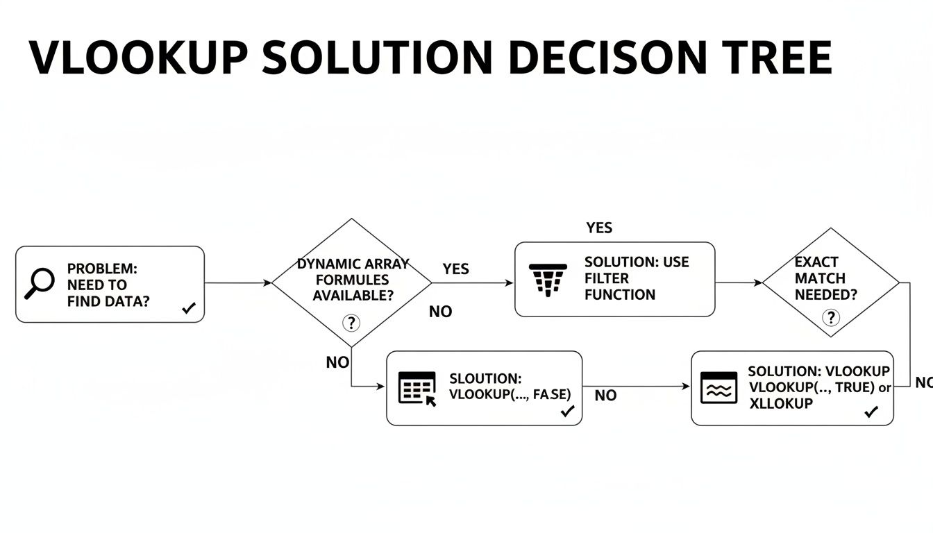
As you can see, if you have access to dynamic arrays (which are standard in modern Excel and Google Sheets), the FILTER function is your most direct route. Knowing what tools you have at your disposal is the first step to moving past VLOOKUP’s limitations.
For a quick reference, here’s a simple table comparing the main methods for returning multiple results.
Quick Guide to Finding Multiple Matches
| Method | Best For | Platform | Ease of Use |
|---|---|---|---|
| FILTER | Simplicity and direct results | Modern Excel, Google Sheets | Very Easy |
| QUERY | Complex filtering, sorting, and aggregating | Google Sheets | Moderate |
| INDEX/SMALL/ROW | Backwards compatibility | Older Excel Versions | Difficult |
Ultimately, picking the right method comes down to your specific needs and the spreadsheet environment you're working in. The good news is, you have powerful options that leave VLOOKUP's single-match limitation in the dust.
The Easiest Way: Using The FILTER Function
When you need to pull every matching result for a lookup, the FILTER function is your new best friend. It’s available in modern Excel versions and Google Sheets, and it's by far the most direct way to get the job done.
Honestly, it feels like this function was designed specifically to solve the old VLOOKUP limitation. It does exactly what the name suggests: it filters a range of data based on a rule you give it and spills all the matching entries. No more clunky, nested formulas.
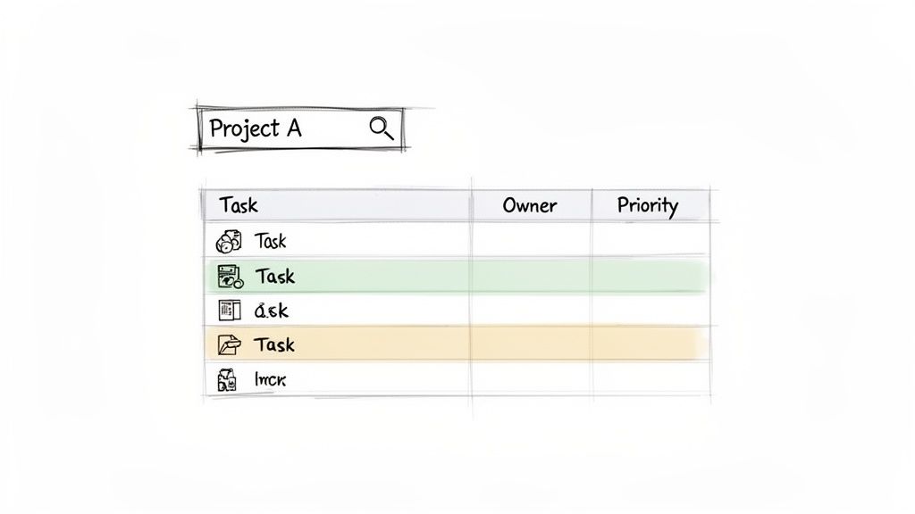
Let's say you have a master list of company tasks. You want to pull a list of every single task assigned to "Project Phoenix." A classic VLOOKUP would stop after finding the first match. FILTER grabs all of them in one clean shot.
How The FILTER Syntax Works
The best part about FILTER is how intuitive its structure is. At its core, the formula looks like this:
=FILTER(range_to_return, condition_range = "your_criteria")
Let's quickly unpack that:
range_to_return: This is the data you actually want to see. It could be a single column with just the task names, or it could be multiple columns with tasks, owners, and due dates.condition_range: This is the column you're searching through. In our example, it would be the column containing all the project names."your_criteria": This is the specific thing you're looking for, like the text "Project Phoenix".
This simple layout makes your formulas easy to read and debug, which is a lifesaver when you come back to a sheet months later.
Dealing With No Matches And Multiple Conditions
So what happens if "Project Phoenix" has no tasks assigned? By default, FILTER throws an error. Thankfully, it has an optional argument built right in to handle this gracefully. You can just add a message to display if the filter comes up empty.
For instance:
=FILTER(A2:C100, B2:B100="Project Phoenix", "No tasks found")
Instead of a jarring #N/A!, your spreadsheet now shows a helpful "No tasks found" message. It’s a small detail that makes your work look much more professional.
Pro Tip: You can also stack multiple conditions to get really specific. Just wrap each condition in parentheses and join them with a multiplication sign (
*), which tells the formula that both conditions must be true.
Let's say you want to find all tasks for "Project Phoenix" that are also marked 'High Priority'. Your formula just needs a small addition:
=FILTER(A2:C100, (B2:B100="Project Phoenix") * (C2:C100="High Priority"))
This ability to layer conditions is what makes FILTER so powerful for building dynamic reports. If you want to explore more ways to combine functions, you can find a lot more in our other guides on advanced Sheets formulas.
Ultimately, FILTER is the modern, clean, and highly effective solution for getting all the matching results you need, minus the headache.
Advanced Lookups With The QUERY Function
If you're a Google Sheets user, at some point you'll hit the limits of basic lookups and discover the QUERY function. Honestly, it's a complete game-changer. Think of it less like a function and more like a mini database language built right into your spreadsheet. It’s a true Swiss Army knife for pulling, sorting, and even calculating data all in one go.
If FILTER is like a simple net that grabs everything matching your criteria, QUERY is more like a high-tech fishing rod. You get to pick the exact lure (SELECT), decide the depth (WHERE), and even specify the size of the fish you want to keep (LIMIT). This is the kind of control you need when building dynamic dashboards or reports without cluttering your sheet with helper columns.
Decoding The QUERY Formula
The syntax looks a bit intimidating at first, mostly because it doesn't feel like a typical spreadsheet function. But once you see the pattern, it's incredibly logical. Let's say you have a big sales log and need to find every deal closed by "Anna" that was over $500.
The basic structure always follows this logic:
=QUERY(data_range, "SELECT columns_to_return WHERE condition")
Using a real-world data range of A1:D100, the formula would look like this:
=QUERY(A1:D100, "SELECT A, D WHERE B = 'Anna' AND D > 500")
Here’s what you’re telling Google Sheets to do: "Look at my data in A1:D100. I only want to see columns A (maybe a Transaction ID) and D (the Sale Amount). And only show me the rows where column B (the Salesperson) is exactly 'Anna' and the value in column D is more than 500."
Key Takeaway: The magic of
QUERYis how it combines these instructions. You’re not just finding matches; you’re specifying what to show, who to look for, and what rules to apply, all in one clean statement.
Adding Advanced Sorting and Limits
But here’s where QUERY really flexes its muscles. You're not just stuck with a raw dump of data; you can organize the results right inside the formula. This is where it leaves other functions in the dust.
Let's build on that last example. What if you want to see Anna's biggest sales at the top of the list? Just add an ORDER BY clause.
- Sorting by Sale Amount: To sort from highest to lowest, you'd add
ORDER BY D DESC(DESC is for descending). - Limiting the Results: If you only care about her top three deals, you can tack on
LIMIT 3at the end.
Putting it all together, you get one elegant formula that does the work of three or four separate steps.
Here’s the final, super-powered version:
=QUERY(A1:D100, "SELECT A, D WHERE B = 'Anna' AND D > 500 ORDER BY D DESC LIMIT 3")
With that single command, you've just asked Sheets to find all of Anna's sales over $500, sort them from largest to smallest, and only give you the top three. It's so much more than just a way to find multiple vlookup results—it's a tool for creating instant, customized reports.
The Classic INDEX SMALL ROW Array Formula

Before we had slick functions like FILTER, getting multiple matches from a lookup was a real head-scratcher. We had to get creative. The go-to solution was a clever, if a bit beastly, combination of INDEX, SMALL, IF, and ROW all bundled into one array formula.
It might look intimidating at first glance, but this formula was the workhorse for returning multiple vlookup results for years. If you ever find yourself working in an older version of Excel that doesn't have dynamic arrays, this old-school method is your best friend. Honestly, learning it is a rite of passage—it really deepens your understanding of how array formulas think.
Breaking Down The Formula's Logic
Think of this formula as a four-part machine, where each function has a specific job to do. Let's say you have a master list of employees and you need to pull out everyone who works in the "Marketing" department.
Here's the play-by-play of what's happening under the hood:
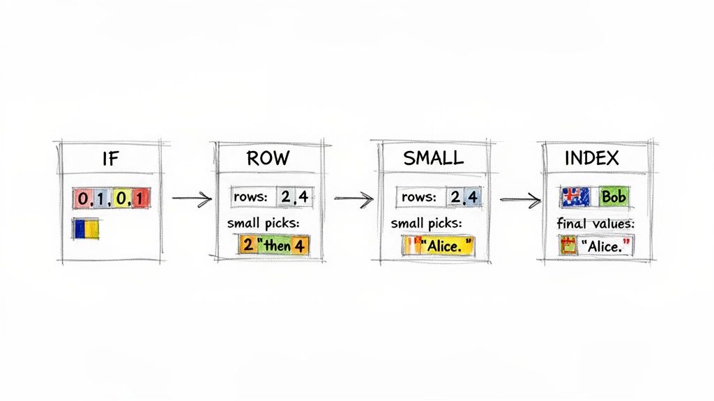
IF: First, theIFfunction scans the department column. It looks at every single cell and asks, "Does this say 'Marketing'?"ROW: WheneverIFgets a "yes," theROWfunction jumps in and grabs that cell's row number.SMALL: Now you have a list of all the row numbers where "Marketing" appears.SMALLtakes this list and sorts it from the lowest number to the highest.INDEX: Finally,INDEXtakes those sorted row numbers one by one and uses them to fetch the actual employee names from their exact positions.
It's this elegant chain reaction that allows you to pull every single matching record from your data, no matter where it's buried in the list.
Building The Array Formula Step-By-Step
Alright, let's put this into practice. Imagine your employee names are in A2:A100 and their departments are in B2:B100. The department we're searching for, "Marketing," is in cell D2.
The formula you'll build looks like this:
{=INDEX(A:A, SMALL(IF($B$2:$B$100=$D$2, ROW($B$2:$B$100)), ROW(1:1)))}
Let's dissect that middle part. The IF statement is the core; it builds a temporary array of row numbers for every match and leaves FALSE for everything else. The ROW(1:1) piece is a neat little trick that acts as a counter. When you drag the formula down, it becomes ROW(2:2), ROW(3:3), and so on, telling SMALL to get the 1st smallest row, then the 2nd smallest, then the 3rd. INDEX just takes that row number and returns the value from column A.
Crucial Note for Excel Users: This is an array formula, so you can't just hit Enter. You have to commit it by pressing Ctrl+Shift+Enter. You’ll know you did it right when Excel wraps the formula in curly braces
{}for you.
This technique is a huge leap from doing things by hand. Manual lookups are incredibly slow—professionals using them average just 2.3 successful lookups per minute. In sharp contrast, automated approaches that can pull multiple results can hit up to 47 lookups per minute. If you want to see the real-world impact of lookup automation, it's worth exploring these operational challenges. While this classic formula requires a bit more setup, it’s a massive step towards that kind of efficiency.
Managing Lookups In Very Large Spreadsheets
When you jump from working with a few thousand rows to a few hundred thousand, the game completely changes. The powerful array formulas we love, like FILTER and QUERY, can suddenly bring your spreadsheet to a grinding halt. Every calculation adds to your browser's workload, and it doesn't take long to get that dreaded "Page Unresponsive" error.
This happens because the formula has to meticulously scan every single cell in your specified range to find what it's looking for. With 500,000 rows, a simple FILTER isn't just a quick lookup anymore; it becomes a massive data processing task happening right inside your browser. This is especially true for the more complex, classic methods like INDEX/SMALL/ROW.
Strategies For Better Performance
To keep your sheet from freezing up, you need to get strategic. The main goal is always to reduce the amount of work your formulas have to do. One of the most effective ways I've found to do this is to isolate your lookup operations.
Instead of pointing a heavy-duty formula at your main, messy data tab, try creating a separate, clean tab. On this new sheet, import only the columns you absolutely need for the lookup. This dramatically shrinks the dataset your formula has to scan, which can give you a huge speed boost. For example, if your master sheet has 26 columns but you just need to find a name in column B and pull a corresponding ID from column A, your new tab should only contain those two columns.
Your primary goal with large datasets is to minimize calculation load. By pre-filtering data on a separate sheet or using helper columns, you reduce the number of cells your formulas must process, making your lookups much faster and more reliable.
Another fantastic tactic is to use helper columns. You can offload parts of a complex formula into a separate column first. Let's say your criteria involve checking two conditions, like Department = "Sales" AND Status = "Active". You could create a helper column with a simple formula like =AND(B2="Sales", C2="Active"). This gives you a clean column of TRUE or FALSE values. Now, your final FILTER formula just has to look for TRUE in that one column, which is far more efficient.
When Your Data Is Too Big For The Browser
Sooner or later, you'll hit a wall where no amount of formula optimization is enough. Google Sheets has its limits, and trying to wrangle millions of rows directly in a browser is often an exercise in futility. If you want to dive deeper into these limitations, you can read our guide on the Google Sheets row limit.
When you're dealing with data at that scale, the best approach is to move the processing to a server-side tool. Services like SmoothSheet are built for exactly this scenario. They handle massive file imports by processing the data on a powerful server before it ever touches your browser. This method completely sidesteps browser freezes and lets you work with millions of rows without crashing your computer. It’s all about letting the right tool do the heavy lifting.
Answering Your Top Questions About Multiple VLOOKUP Results
Even with powerful functions like FILTER and QUERY in your toolkit, you'll inevitably hit a few roadblocks when trying to pull multiple matches. These functions are incredibly flexible, but some real-world scenarios require a bit more creativity.
Let's dive into the common questions I hear all the time: condensing results into one cell, dealing with massive datasets, and pulling information from other spreadsheets. These are the practical problems you run into right after you've nailed the basics.
How Can I Get All My Results in a Single Cell?
Sometimes, you don't want results spilling down multiple rows. A clean, comma-separated list in one cell is much better for a dashboard or summary view. The trick is to pair your multi-result formula with a function that joins text together.
In Google Sheets, TEXTJOIN is your best friend for this. It’s a simple, two-step process:
- First, use a function like
FILTERorQUERYto generate the list of matches. - Then, wrap that entire formula inside
TEXTJOIN.
Let’s say you want a list of all tasks for "Project Phoenix" in a single cell. The formula would be:
=TEXTJOIN(", ", TRUE, FILTER(A:A, B:B="Project Phoenix"))
Here, ", " is the separator you want between each task, TRUE tells the function to ignore any blank cells it finds, and the FILTER part hands over the list of results. It's a surprisingly simple way to get a much cleaner output.
Which Method Is Best for Huge Datasets?
When your spreadsheet balloons to tens of thousands of rows, performance becomes a serious issue. For truly massive datasets (50,000+ rows), Google Sheets' QUERY function is almost always the winner. Its processing is handled on Google's powerful servers, making it far more efficient than functions that rely on your local browser's resources.
On the other hand, the classic INDEX/SMALL/ROW array formula, while clever, is typically the slowest. It can set off a chain reaction of recalculations that brings large sheets to a crawl. FILTER is a great, modern alternative, but even it can start to lag if you're working with enormous ranges and multiple complex conditions.
The single best thing you can do for performance is to reduce the amount of data your formulas have to scan. I often create a dedicated tab with pre-filtered data. This one move can dramatically speed up your lookups and make your entire sheet more responsive.
This isn't just a theoretical problem. A major challenge for 67% of enterprises is pulling lookup data from specific historical points in time, like monthly project snapshots. In one case, project managers were spending about six hours every month manually digging through cell history to find old data—a task a well-built lookup could automate in seconds. You can see how companies are trying to solve historical data lookups in real-world scenarios.
Can I Pull Multiple Results From a Different Spreadsheet?
You sure can. All the methods we've discussed can work across separate spreadsheets by bringing IMPORTRANGE into the mix. You just use IMPORTRANGE inside your main formula to define the source URL and data range.
For instance, here’s how you’d use FILTER to pull data from another file:
=FILTER(IMPORTRANGE("URL", "Sheet1!A:A"), IMPORTRANGE("URL", "Sheet1!B:B") = "criteria")
This is an incredibly powerful way to connect data across your organization, but a word of caution: use it judiciously. Every IMPORTRANGE creates a live link between files. Piling on too many of them, especially from large source sheets, will drastically slow down your spreadsheet's load times and calculations. If you start seeing errors, our guide on using IFERROR in Google Sheets can help you manage them without breaking your sheet.
When your files get so big that formulas lag and your browser freezes, it's time to upgrade your tools. SmoothSheet lets you import massive CSV and Excel files right into Google Sheets without the hang-ups. It processes the heavy data on a server, so you can work with millions of rows like it’s nothing. Get started with SmoothSheet for free.