
If you've ever spent time dragging a formula down hundreds (or thousands) of rows in Google Sheets, you already know the pain. Copy, paste, scroll, repeat. There's a better way: ARRAYFORMULA in Google Sheets lets you apply a single formula to an entire column instantly. No dragging, no duplicating, no manual row-by-row work. In this guide, you'll learn exactly how ARRAYFORMULA works, see practical examples with IF, VLOOKUP, and conditional logic, and pick up tips to avoid the most common pitfalls.
Key Takeaways:ARRAYFORMULA applies one formula across an entire column or range automaticallyIt can reduce hundreds of individual formulas to a single cell, cutting recalculation time by up to 50%Pair it with IF, VLOOKUP, or SUMIF for powerful bulk operationsUse closed ranges (e.g., A2:A1000) instead of open ranges for better performanceWhen importing large datasets with SmoothSheet, ARRAYFORMULA processes them without row-by-row formulas
What Is ARRAYFORMULA in Google Sheets?
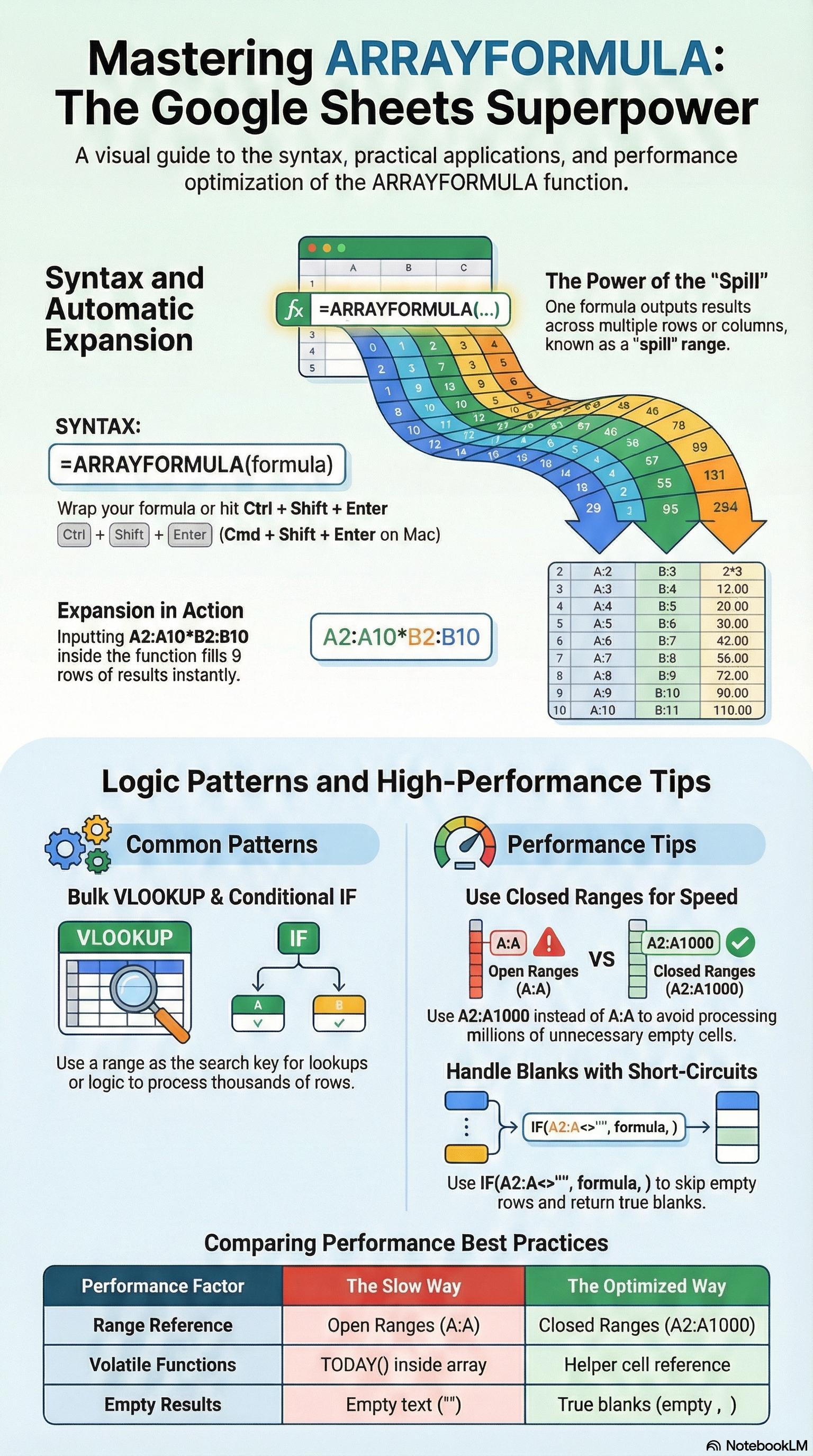
ARRAYFORMULA is a Google Sheets function that takes a formula designed for a single cell and applies it to an entire range of cells at once. Instead of writing the same formula in every row, you write it once, and Google Sheets expands the results automatically. You can find the official syntax reference in the Google Sheets function list.
The syntax is straightforward:
=ARRAYFORMULA(array_formula)Where array_formula is any expression that uses a range instead of a single cell reference. For example, instead of writing =A2*B2 and dragging it down, you write:
=ARRAYFORMULA(A2:A*B2:B)This single formula in one cell fills the entire column with the results. Think of it as telling Google Sheets: "Do this calculation for every row in the range, not just this one."
There's also a handy keyboard shortcut. Type your formula normally and press Ctrl + Shift + Enter (Windows) or Cmd + Shift + Enter (Mac) to automatically wrap it in ARRAYFORMULA.
Why Does This Matter?
In a typical spreadsheet, you might have the same formula copied across 5,000 rows. Each one recalculates independently. With ARRAYFORMULA, a single formula handles all 5,000 rows. This means:
- Fewer formulas = faster spreadsheet performance
- Easier maintenance = change the formula once, it updates everywhere
- Cleaner sheets = no accidental formula overwrites in individual cells
How to Use ARRAYFORMULA (Step-by-Step)
Let's walk through the most common ARRAYFORMULA patterns, starting simple and building up to more advanced combinations.
Basic Example: Apply a Formula to an Entire Column
Say you have product prices in column A and quantities in column B, and you want the total cost in column C. Normally you'd write =A2*B2 in C2 and drag it down. With ARRAYFORMULA:
- Click on cell C2 (the first cell where you want results)
- Enter the formula:
=ARRAYFORMULA(A2:A*B2:B) - Press Enter
That's it. Every row in column C now shows the product of the corresponding A and B cells. When you add new data in rows A and B, the results appear automatically in column C.
Pro tip: If you only want results for rows that actually have data (and not zeros filling empty rows), wrap it with an IF check:
=ARRAYFORMULA(IF(A2:A="", "", A2:A*B2:B))This checks whether column A is empty. If it is, the formula returns a blank instead of zero.
ARRAYFORMULA with IF Statements
Combining ARRAYFORMULA with IF is one of the most useful patterns. It lets you categorize, label, or conditionally calculate across an entire column.
Example 1: Categorize values
Suppose column A contains sales figures and you want to label each as "High" or "Low" based on whether they exceed $2,000:
=ARRAYFORMULA(IF(A2:A > 2000, "High", "Low"))Every row gets its label instantly. No dragging needed.
Example 2: Calculate a bonus only for qualifying sales
If you want to calculate a 10% bonus only for salespeople with revenue above $12,000:
=ARRAYFORMULA(IF(D3:D > 12000, D3:D * 0.1, 0))This returns the bonus amount for qualifying rows and zero for everyone else.
Example 3: Handle blanks gracefully
To avoid showing results for empty rows, nest another IF at the beginning:
=ARRAYFORMULA(IF(A2:A = "", "", IF(A2:A > 2000, "High", "Low")))The outer IF checks for blanks first, so your column stays clean.
ARRAYFORMULA with VLOOKUP
One of the most powerful combinations is ARRAYFORMULA with lookup functions. Instead of running VLOOKUP row by row, you can look up an entire column of values at once.
Say you have order IDs in column D and you want to pull the matching customer names from a reference table in A2:B100:
=ARRAYFORMULA(VLOOKUP(D2:D, A2:B100, 2, FALSE))This performs a VLOOKUP for every value in column D simultaneously. For large datasets — like the ones you might import with SmoothSheet from CSV or Excel files — this is dramatically faster than having individual VLOOKUP formulas in each row.
To handle blanks and errors, wrap it with IFERROR:
=ARRAYFORMULA(IF(D2:D = "", "", IFERROR(VLOOKUP(D2:D, A2:B100, 2, FALSE), "Not Found")))ARRAYFORMULA with Conditional Formatting Logic
While ARRAYFORMULA doesn't directly control conditional formatting (that's a separate Sheets feature), it's extremely useful for creating helper columns that drive conditional formatting rules.
For example, you might create a status column that flags overdue items:
=ARRAYFORMULA(IF(A2:A = "", "", IF(C2:C < TODAY(), "Overdue", "On Track")))Then apply conditional formatting to the helper column: if the cell says "Overdue," highlight it red. This approach is cleaner and faster than writing complex conditional formatting formulas directly.
Note: Be careful with volatile functions like TODAY() inside ARRAYFORMULA. Since TODAY() recalculates constantly, the formula reprocesses on every edit. For better performance, put =TODAY() in a separate cell (say, Z1) and reference that cell instead:
=ARRAYFORMULA(IF(A2:A = "", "", IF(C2:C < $Z$1, "Overdue", "On Track")))When to Use ARRAYFORMULA (And When Not To)
ARRAYFORMULA is powerful, but it's not always the best tool for the job. Here's a practical breakdown.
Use ARRAYFORMULA When:
- You need the same formula in every row — multiplication, concatenation, IF checks, lookups
- Your data grows dynamically — new rows automatically get formulas applied
- You want easier maintenance — one formula to update instead of hundreds
- You're importing large datasets — after pulling data into Sheets with SmoothSheet, ARRAYFORMULA processes entire columns without manual formula dragging
Consider Alternatives When:
- You need to aggregate or group data: The QUERY function is better for SQL-like operations (SUM, COUNT, GROUP BY)
- You need to filter rows: The FILTER function extracts matching rows more efficiently than ARRAYFORMULA + IF
- You're working with 50,000+ rows: Even ARRAYFORMULA can slow down at this scale. Consider whether you really need every row calculated, or if a QUERY or pivot table is more appropriate
Performance Tips
Keep these rules in mind for smooth performance:
- Use closed ranges — Write
A2:A1000instead ofA2:A. Open ranges force Google Sheets to evaluate thousands of empty rows, and this adds up fast. - Avoid volatile functions inside ARRAYFORMULA — Functions like
NOW(),TODAY(), andRAND()recalculate on every edit. Place them in a helper cell and reference it. - Handle blanks with an IF wrapper — Use
IF(A2:A <> "", ...)to skip empty rows. This prevents unnecessary calculations and keeps your output clean. - Check your spreadsheet's cell count — Google Sheets has a 10 million cell limit. If your ARRAYFORMULA outputs span large ranges, make sure you're not approaching that ceiling.
Common ARRAYFORMULA Errors and Fixes
Even experienced Sheets users run into these errors. Here's how to diagnose and fix each one.
#REF! Error (Spill Error)
This is the most common ARRAYFORMULA error. It happens when the formula tries to expand its results into cells that already contain data.
Example: You place an ARRAYFORMULA in C2 that should fill C2:C100, but cell C15 already has a value typed in. The formula can't "spill" past that obstruction, so it throws #REF!.
Fix:
- Clear any values in the cells where the ARRAYFORMULA needs to expand
- Make sure no other formulas are occupying the output range
- Check for invisible characters (spaces) in seemingly empty cells — select the range and press Delete to be sure
Circular Dependency Error
This occurs when the ARRAYFORMULA references a range that includes its own output cell, creating an infinite loop.
Example: You place an ARRAYFORMULA in A1 that references A1:A100. The formula tries to use its own result as input, which creates a circular reference.
Fix:
- Make sure the formula's input range and output range don't overlap
- If you need to reference data in the same column, use a helper column for the ARRAYFORMULA output
- Check for indirect circular references where Cell A depends on Cell B, which depends on Cell A
Formula Returns Only One Result
Sometimes your ARRAYFORMULA only fills one cell instead of the entire range. This usually means you're using a function that doesn't natively support arrays.
Common causes:
- Using
OR()orAND()inside ARRAYFORMULA — these don't expand properly. Use arithmetic equivalents instead:+for OR,*for AND - Referencing a single cell instead of a range —
ARRAYFORMULA(IF(A2 > 10, "Yes", "No"))only checks A2. Change it toA2:A
Unexpected Zeros or Empty Rows
When ARRAYFORMULA processes empty rows, math operations return 0 and text operations may return empty strings that still take up space.
Fix: Always wrap with a blank check:
=ARRAYFORMULA(IF(A2:A = "", "", your_formula_here))Frequently Asked Questions
Can ARRAYFORMULA work with IMPORTRANGE in Google Sheets?
Yes, but with a catch. IMPORTRANGE already returns an array, so you typically don't need to wrap it in ARRAYFORMULA. However, if you want to perform calculations on imported data — like multiplying every value by a rate — you can use ARRAYFORMULA on the imported range. For example: =ARRAYFORMULA(IMPORTRANGE("spreadsheet_url", "Sheet1!A2:A100") * 1.1). Just make sure the IMPORTRANGE has been authorized first by clicking "Allow access" when prompted.
What is the difference between ARRAYFORMULA and dragging a formula down?
Dragging a formula creates an independent copy in every cell. If you have 5,000 rows, that's 5,000 separate formulas recalculating individually. ARRAYFORMULA uses a single formula in one cell that outputs results to the entire range. This means faster recalculation, easier editing (change it in one place), and automatic coverage of new rows. The tradeoff is that you can't customize the formula for individual rows — it applies the same logic everywhere.
Why is my ARRAYFORMULA slow in Google Sheets?
The most common cause is using open-ended ranges like A2:A, which forces Sheets to evaluate every row in the column — even empty ones. Switch to closed ranges like A2:A5000. Also check for volatile functions (TODAY(), NOW(), RAND()) nested inside the ARRAYFORMULA, as these trigger constant recalculation. Finally, avoid nesting multiple ARRAYFORMULAs that reference each other — this creates cascading recalculations that can grind your sheet to a halt.
Does ARRAYFORMULA automatically apply to new rows?
Yes, if you use an open-ended range like A2:A, the formula automatically covers any new rows you add. If you use a closed range like A2:A100, new data in row 101 won't be included — you'd need to extend the range. For dynamic coverage, open ranges are convenient but come with the performance cost of processing empty rows. A good compromise is to use a generously sized closed range (e.g., A2:A10000) with an IF blank check to skip empty rows.
Conclusion
ARRAYFORMULA is one of those Google Sheets features that, once you learn it, you'll wonder how you ever managed without it. A single formula in one cell can replace hundreds of individual formulas, making your spreadsheets faster, cleaner, and easier to maintain.
Start with the basics — a simple multiplication or IF statement across a column — and work your way up to combining it with VLOOKUP, SUMIF, or other functions. Just remember the golden rules: use closed ranges for performance, handle blanks with IF wrappers, and watch out for spill errors.
And if your workflow involves importing large CSV or Excel files into Google Sheets before applying these formulas, SmoothSheet handles the heavy lifting with server-side processing — so your browser doesn't crash before you even get to the formula stage. Give it a try at $9/month.