
Knowing how to freeze rows and columns in Google Sheets is one of those skills that seems small but makes a huge difference. It’s all about locking your headers in place so they stay visible while you scroll. This way, you never lose your spot or have to guess what you're looking at, which honestly saves a ton of time and prevents silly mistakes.
Your Go-To Trick for Big Spreadsheets
Ever found yourself scrolling deep into a massive spreadsheet, only to completely forget what column G was supposed to be? Was it "Revenue" or "Units Sold"? We've all been there, scrolling back and forth like a maniac just to check the header. Freezing panes fixes that headache for good.
Think about managing a project task list with hundreds, or even thousands, of entries. If you freeze that top row with your headers—"Task Name," "Due Date," "Assigned To"—you can glide through the entire list without ever losing context. It turns what could be a messy data review into a surprisingly smooth process.
Work Faster and Keep Your Team on the Same Page
This isn't just a solo productivity hack. With 1.1 billion users worldwide, Google Sheets is where teams get work done together. When you lock the headers, you're giving everyone who opens that sheet the same clear frame of reference. It cuts down on confusion and makes sure the data stays accurate for the whole team.
This becomes absolutely essential when you're prepping data for analysis. Let's say you're getting a big dataset organized before you dive in.
By keeping your main headers or key identifiers locked and visible, you make sure your analysis is spot-on from the get-go. It’s a foundational step for more powerful features, like building a solid pivot table in Google Sheets.
When it comes down to it, getting the hang of freezing panes is a simple way to level up your spreadsheet game. You’ll work faster, make fewer errors, and be a much more effective collaborator.
The 2 Quickest Ways to Freeze Rows and Columns on Desktop
When you’re staring at a massive spreadsheet, the last thing you want is to lose track of your headers. Keeping that context in view is crucial, and thankfully, Google Sheets gives you a couple of incredibly simple ways to lock down rows and columns on your computer.
You can either use a quick drag-and-drop for a visual fix or go through the top menu for more precise control. Both get the job done, turning a scrolling nightmare into a manageable task.
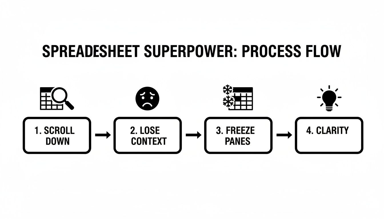
The image above really nails the problem: scrolling without frozen panes leads to confusion, but locking them brings back instant clarity.
The Drag-and-Drop Method
For a fast, intuitive way to freeze panes, the drag-and-drop method is your go-to. It's my personal favorite for quick adjustments.
Just look in the very top-left corner of your sheet. You’ll see two slightly thicker gray bars—one just above row 1 and another to the left of column A. These are the handles.
Hover your mouse over the horizontal bar until the cursor turns into a hand icon. Then, just click and drag it down over the rows you want to freeze. Let go, and they're locked. It works the same way for columns—grab the vertical bar and pull it to the right.
This technique is perfect for common tasks. Need to lock your main header? Just drag the bar down one row. Working with a grade book? Drag the vertical bar to the right to keep student names visible as you scroll through their assignments. I've found it's the fastest way to prevent that "wait, whose score is this?" moment.
The View Menu Method
If you prefer using menus or need to freeze a specific, larger number of rows and columns, the View menu is your best bet. It feels a bit more formal but offers pinpoint accuracy.
Here's how it works:
- First, click any cell in your sheet to make sure it's active.
- Go to the top menu and click View.
- Hover your cursor over Freeze.
- A new menu will pop out with a few preset options.
You can instantly choose to freeze up to 2 rows or 2 columns.
Pro Tip: Need to freeze more than two of each? Here’s the trick. Click the one cell that is just below the last row you want to freeze and to the right of the last column you want to freeze. Now, go to View > Freeze. The options will automatically update to let you freeze everything above and to the left of your selection. It's a game-changer for complex sheets.
Desktop Freeze Methods At a Glance
Still not sure which method is right for you? This table breaks it down.
| Method | Best For | Steps | Pro Tip |
|---|---|---|---|
| Drag-and-Drop | Quick, visual adjustments for 1-2 rows/columns. | Hover over the gray bar in the top-left corner until a hand icon appears, then drag and release. | Best for simple headers and sidebars where precision isn't critical. |
| View Menu | Precise control, especially for freezing multiple rows and columns at once. | Select a cell, then navigate to View > Freeze and choose an option. | To freeze custom ranges, select the cell below and to the right of your desired freeze area first. |
Both methods are incredibly useful. I tend to use the drag-and-drop for everyday tasks but switch to the View menu when I’m setting up a complex new report that needs a specific layout from the start. You can learn more practical tips by reading the full guide on how to freeze panes on SheetAI.app.
How to Freeze Panes on Your Mobile Device
Let's be honest, working with big spreadsheets on a phone can be a real pain. But thankfully, the Google Sheets mobile app makes it surprisingly simple to keep your bearings. Freezing your headers is just a few taps away, so you'll always know what you're looking at, no matter how far down you scroll.
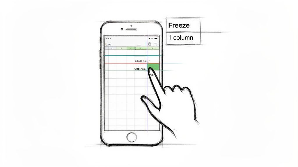
The method works the same whether you're on an Android or an iPhone. Forget about dragging bars like you do on a computer; the mobile app uses a simple tap-and-hold approach.
To get started, just tap the header of the row or column you want to lock. For instance, tap the number 1 to select that entire first row.
Locking Your View on the Go
With the row or column highlighted, tap it again. A little context menu will pop up with familiar options like "Cut," "Copy," and "Paste."
On the far right of that menu, tap the three-dot icon to see more options. A quick scroll will reveal the Freeze button—give it a tap. That's it! Your selection is now locked, marked by a slightly thicker gray line.
To undo it, just follow the same steps and tap Unfreeze instead.
Since its refinement, mobile freezing has become a key feature for freelancers and marketing teams tracking extensive data on the go. While desktop users often prefer the speed of dragging freeze bars, the mobile tap-and-select method is exceptionally smooth and avoids the common desktop error of over-freezing. Discover more insights on these workflow differences at KieranDixon.com.
A quick tip for mobile: since you're working with such a small screen, be selective. Freezing just the top header row or the first column is usually the sweet spot. It gives you enough context to understand your data without making the sheet feel cramped and unusable.
Common Problems and How to Fix Them
Even a simple feature like freezing panes can misbehave now and then. You might see the freeze line pop up in a weird spot or find it won't lock at all, especially after dumping a huge amount of data into your sheet. Don't worry, these are usually quick fixes.
Most of the time, issues with freezing panes come down to a misplaced click or a simple browser hiccup. Let’s walk through the most common headaches so you can get your spreadsheet back in order.
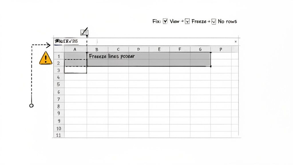
Freeze Line Appears in the Wrong Place
This is probably the most common issue I see. You accidentally freeze way too many rows or columns, and suddenly you can barely scroll through your data. It usually happens with a stray click-and-drag.
Thankfully, the fix is easy. Just move your cursor over the thick gray freeze line until it changes into a little hand icon. Then, simply click and drag the line all the way back to the top-left corner of your sheet. That’s it—the freeze is gone.
If you prefer using the menu, you can do a clean reset this way:
- Head up to View > Freeze.
- Choose No rows and then follow up with No columns.
Doing both ensures any lingering freeze settings are totally cleared out, giving you a fresh start.
A classic mistake is selecting a cell deep in your data before you hit "Freeze." Always remember: Google Sheets locks everything above and to the left of your active cell. Make sure you click the cell just below the last row and to the right of the last column you want to keep visible.
Panes Won’t Lock After a Large Data Import
Ever import a massive CSV or Excel file and find that Google Sheets suddenly feels a bit sluggish? Sometimes, in these situations, the freeze pane feature just stops responding, or the lines don't show up when you try to apply them.
Your first move should always be a quick page refresh (Ctrl + R on Windows, Cmd + R on Mac). More often than not, this clears up a temporary browser cache issue that's getting in the way.
If a refresh doesn't do the trick, the file size itself could be the problem. When a sheet gets too bloated, its performance can really suffer. If this is a recurring problem for you, it might be time to look into our guide on how to fix the "file too large" error in Google Sheets for some longer-term solutions.
Working with Large and Collaborative Sheets
Knowing how to freeze a row is one thing, but when you're working in a massive or shared spreadsheet, a little strategy goes a long way. The biggest thing to remember is that when you freeze panes, it affects everyone who has the sheet open.
This is why, for any kind of teamwork, Filter Views are almost always a better option. They let each person sort and filter the data to their own liking without messing up the view for everyone else. No more frantic Slack messages asking who broke the sorting!
Freezing More Complex Headers
What if your headers are more complex, with a main category in one row and sub-categories in the row below it? You can’t just freeze the top row; you need to lock the entire header block so you don't lose context.
The fix is simple: just drag the gray freeze bar down to cover all your header rows. If you have a 3-row header, for example, you'll drag the bar to sit just below row 3. This locks the entire block in place, keeping the full context visible while you scroll through your data.
Keep in mind that performance can take a hit on seriously large sheets. When a file has hundreds of thousands of cells, even basic actions like freezing rows can make your browser lag. A clean, well-organized sheet is your best defense.
Pushing a spreadsheet to its limits can test your browser's patience. If you're running into constant slowdowns, it might be a sign you're nearing a hard limit. You can check where your sheet stands with this helpful Google Sheets limits calculator to see if you're getting close to any thresholds.
Common Questions About Freezing Panes in Google Sheets
As you get the hang of freezing rows and columns, a few questions tend to come up again and again. Let's tackle some of the most common ones so you can get back to your data without a hitch.
Can I Freeze a Row in the Middle of My Sheet?
Unfortunately, no. Google Sheets is pretty strict on this one—you can only freeze rows starting from the very top and columns from the far left. You can't just pick a row out of the middle of your dataset and lock it in place.
If you have a crucial piece of information floating in the middle of your sheet that you need to keep an eye on, the best workaround is to simply move those rows to the top.
How Do I Unfreeze Everything?
Getting rid of frozen panes is just as easy as setting them up. The most direct method is to grab the thick gray line that marks your frozen area and just drag it all the way back to the top-left corner of your sheet.
You can also head back to the menu. Just go to View > Freeze and select either No rows or No columns to clear the settings.
This is my go-to "reset button." If I've frozen the wrong section or just want a clean slate, popping into the menu to select 'No rows' is the quickest way to start over.
Why Is the Freeze Option Grayed Out?
This is a classic problem, and it usually boils down to one of two things.
First, check your selection. The freeze function gets confused if you have multiple, separate cells selected. Make sure you’ve only clicked on a single cell before you try to freeze anything.
The other culprit is often protected ranges. If the cells you're trying to work with are part of a protected area and you don't have editing permissions, Google Sheets won't let you apply a freeze.
If neither of those is the issue, a quick refresh of the page can often clear up any weird, temporary glitches. And if you're wrangling a massive dataset, sometimes Sheets just gets a little sluggish. You might find our guide on the official Google Sheets row limit helpful for understanding those boundaries.
Tired of your browser freezing before your panes do? SmoothSheet lets you import massive CSV and Excel files directly into Google Sheets without crashes or row limits. Our server-side processing handles millions of rows in the background, so you can keep working while we do the heavy lifting. Try SmoothSheet for free and import your large files in minutes.