
The FILTER function in Google Sheets lets you pull exactly the rows you need from a dataset — no manual sorting, no helper columns, no clunky menus. Unlike the built-in filter views that alter how your sheet looks, the FILTER function returns a dynamic, formula-driven subset of your data that updates automatically when your source changes.
Whether you are sifting through sales records by region, extracting overdue invoices, or building a dashboard that responds to dropdown selections, FILTER is the function that makes it happen. In this guide, you will learn the syntax, see real examples with multiple conditions, and discover how to combine FILTER with SORT, UNIQUE, and IFERROR for production-ready formulas.
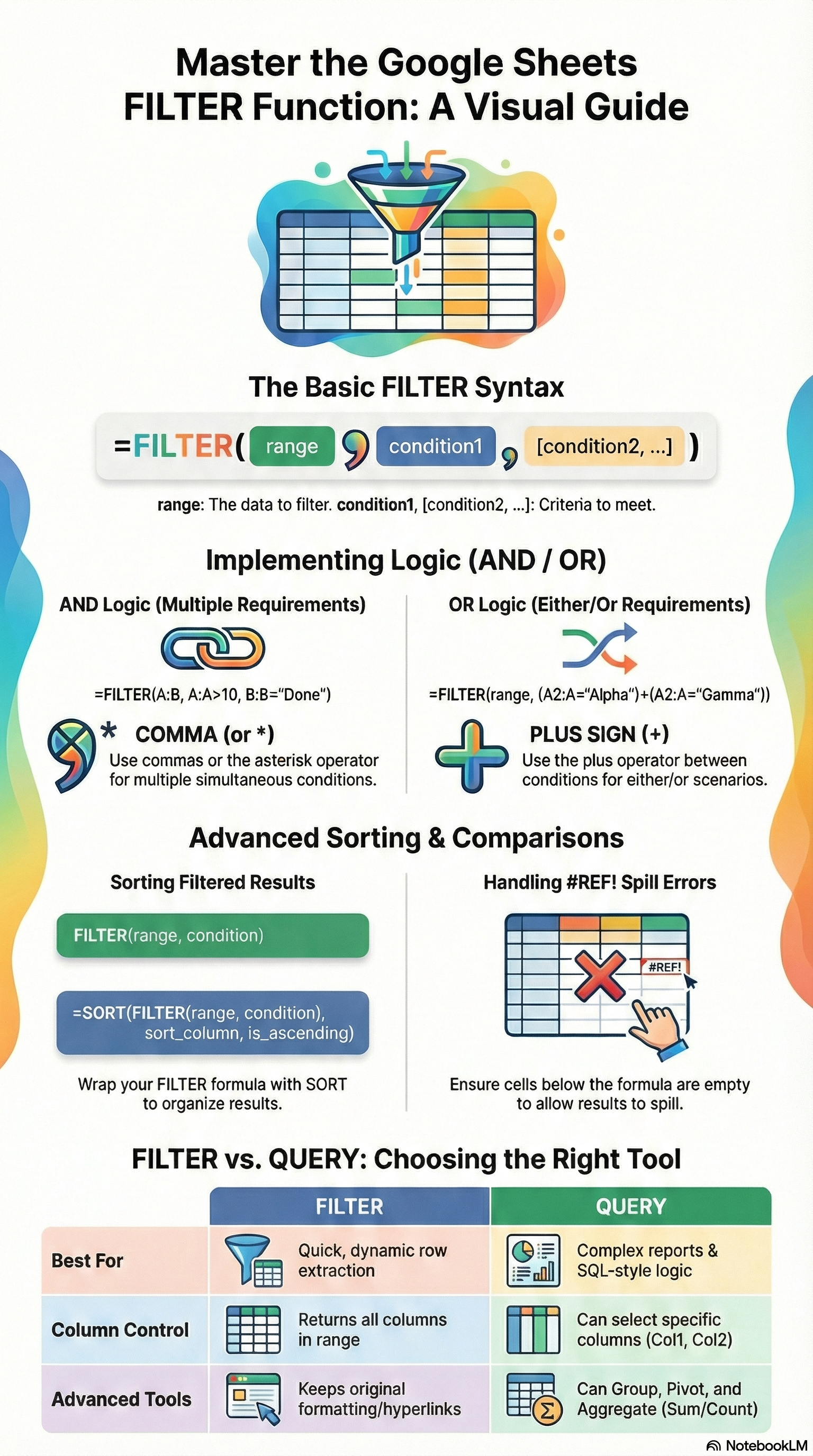
Key Takeaways:FILTER dynamically extracts rows matching one or more conditions — no helper columns neededUse*for AND logic and+for OR logic when combining multiple conditionsWrap FILTER with SORT, UNIQUE, or IFERROR to build advanced, error-proof formulasFILTER is faster and simpler than QUERY for straightforward row extractionWhen your CSV source exceeds 100K rows, SmoothSheet imports it server-side so your FILTER formulas have clean data to work with
FILTER Function Syntax
The FILTER function follows a straightforward pattern:
=FILTER(range, condition1, [condition2, ...])| Parameter | Required | Description |
|---|---|---|
range | Yes | The data you want to filter (e.g., A2:E100) |
condition1 | Yes | A Boolean array or expression the same height as range |
condition2, ... | No | Additional conditions — all must be TRUE for a row to appear (AND logic) |
A few rules to keep in mind:
- Every condition must produce an array of TRUE/FALSE values that matches the number of rows in
range. - When you list multiple conditions separated by commas, Google Sheets treats them as AND — every condition must be true.
- If no rows match, FILTER returns
#N/A. We will cover how to handle that with IFERROR later in this guide.
FILTER Examples
Basic: Filter Rows by One Condition
Imagine you have a sales table in A1:D20 with columns for Name, Region, Product, and Amount. To extract only the rows where Region equals "West":
=FILTER(A2:D20, B2:B20="West")This returns every column (A through D) for rows where column B contains "West". The result spills into adjacent cells automatically — no dragging required.
You can also use comparison operators. To find all sales above $5,000:
=FILTER(A2:D20, D2:D20>5000)Multiple Conditions (AND with *, OR with +)
AND logic — comma method: List conditions as separate arguments. Both must be true:
=FILTER(A2:D20, B2:B20="West", D2:D20>5000)This returns rows where the region is "West" and the amount exceeds $5,000.
AND logic — multiplication method: Multiply Boolean arrays with *. The result is the same, but this syntax is useful when you need to nest conditions inside other functions:
=FILTER(A2:D20, (B2:B20="West") * (D2:D20>5000))OR logic — addition method: Add Boolean arrays with +. A row appears if either condition is true:
=FILTER(A2:D20, (B2:B20="West") + (B2:B20="East"))This returns rows where the region is "West" or "East". The + operator treats any non-zero value as TRUE, which is exactly how Boolean OR works.
FILTER with SORT
FILTER extracts the rows; SORT orders them. Wrap FILTER inside SORT to get a sorted, filtered result in one formula:
=SORT(FILTER(A2:D20, B2:B20="West"), 4, FALSE)This filters for "West" and sorts the results by the 4th column (Amount) in descending order. The FALSE parameter means descending; use TRUE for ascending.
You can also sort by multiple columns:
=SORT(FILTER(A2:D20, D2:D20>1000), 2, TRUE, 4, FALSE)This filters rows above $1,000, then sorts first by column 2 (Region, A-Z) and then by column 4 (Amount, highest first).
FILTER with UNIQUE for Distinct Values
Need a deduplicated list from your filtered results? Wrap FILTER inside UNIQUE:
=UNIQUE(FILTER(C2:C20, B2:B20="West"))This returns the distinct product names sold in the "West" region — no duplicates. This combination is especially powerful when building data validation dropdowns or summary tables.
FILTER vs QUERY: Which Should You Use?
Both FILTER and QUERY can extract subsets of data, but they work very differently under the hood. Here is a quick comparison to help you choose:
| Feature | FILTER | QUERY |
|---|---|---|
| Syntax style | Standard spreadsheet formula | SQL-like string (SELECT... WHERE...) |
| Learning curve | Low — if you know IF, you know FILTER | Medium — requires learning Google Visualization API Query Language |
| Select specific columns | Requires helper like INDEX or CHOOSECOLS | Built-in with SELECT clause |
| Aggregation (SUM, AVG, COUNT) | Not built-in — needs wrapping with SUM, etc. | Built-in with GROUP BY |
| Multiple conditions | Comma-separated or * / + operators | WHERE... AND... OR... |
| Sorting | Wrap with SORT() | Built-in with ORDER BY |
| Pivoting data | Not supported | Built-in with PIVOT |
| Speed on large datasets | Faster for simple filtering | Faster when aggregating |
| Nesting with other functions | Excellent — works inside SORT, UNIQUE, INDEX, etc. | Limited — harder to nest |
Rule of thumb: Use FILTER when you need to extract complete rows based on conditions. Use QUERY when you need to aggregate, group, or select specific columns in a single step. For most day-to-day tasks — pulling records, feeding dashboards, building dependent dropdowns — FILTER is the faster, more readable choice.
If you are new to QUERY, our Google Sheets QUERY function guide walks through the syntax step by step.
Advanced FILTER Techniques
Dynamic Dropdowns with FILTER
One of the most practical uses of FILTER is building sheets that respond to user input. Here is the pattern:
- Create a data validation dropdown in cell
G1with your region options (West, East, North, South). - In cell
G3, enter the FILTER formula referencing that dropdown:
=FILTER(A2:D20, B2:B20=G1)Now whenever someone selects a region from the dropdown, the filtered table updates instantly. No VBA, no scripts, no button clicks.
You can take this further with cascading dropdowns. For example, filter products based on the selected region, then use that filtered product list as the source for a second dropdown. This is how you build interactive mini-dashboards entirely with formulas.
When the dataset behind your dropdown comes from a large CSV or Excel file, SmoothSheet handles the import server-side — so your FILTER formulas reference clean, complete data without browser slowdowns.
FILTER Across Sheets
FILTER works seamlessly with cross-sheet references. If your raw data lives on a sheet called "Data" and you want filtered results on a "Dashboard" sheet:
=FILTER(Data!A2:D500, Data!B2:B500="West")This is especially useful when you keep raw imported data on one tab and build reports on another. If you are pulling data from entirely separate spreadsheets, combine FILTER with INDEX MATCH or IMPORTRANGE for cross-file lookups.
Handling #N/A When No Results (IFERROR Wrapper)
When no rows match your FILTER conditions, Google Sheets returns a #N/A error with the message "FILTER has no matches." This can break downstream formulas and looks unprofessional in shared sheets.
The fix is simple — wrap FILTER with IFERROR:
=IFERROR(FILTER(A2:D20, B2:B20="Antarctica"), "No matching records found")You can return any fallback value: an empty string (""), a message, or even a default dataset. For more error-handling patterns, check our guide on ARRAYFORMULA in Google Sheets, which covers IFERROR in array contexts.
FAQ
Can the FILTER function handle more than two conditions?
Yes. You can add as many conditions as you need, either as separate comma-separated arguments (AND logic) or combined with * and + operators. For example, =FILTER(A2:D20, B2:B20="West", C2:C20="Widget", D2:D20>1000) applies three AND conditions. There is no hard limit on the number of conditions.
Why does my FILTER formula return #N/A?
FILTER returns #N/A when no rows in your dataset match all of the specified conditions. This is expected behavior, not a formula error. Wrap your formula with IFERROR to display a custom message or empty result instead: =IFERROR(FILTER(...), "No results").
Is FILTER faster than QUERY for large datasets?
For simple row extraction, FILTER is generally faster because it uses native array operations without parsing a query string. However, if you need aggregation (SUM, COUNT, AVG) or column selection, QUERY can be faster since it handles everything in one pass. For datasets over 50,000 rows, performance depends more on your sheet's overall complexity than the function choice. If your source CSV is very large, use SmoothSheet's CSV Splitter to break it into manageable chunks before importing.
Can I use FILTER with ARRAYFORMULA?
FILTER already returns an array, so you typically do not need to wrap it with ARRAYFORMULA. However, you can use FILTER inside ARRAYFORMULA when combining it with other functions that need array expansion. For instance, =ARRAYFORMULA(LEN(FILTER(A2:A20, B2:B20="West"))) returns the character length of each filtered value. In most cases, FILTER handles array output on its own.
Conclusion
The FILTER function is one of the most versatile tools in Google Sheets. It replaces manual filter views with dynamic, formula-driven results that update automatically. Combined with SORT, UNIQUE, and IFERROR, it handles everything from simple lookups to interactive dashboards — all without scripts or add-ons.
Start with a basic single-condition FILTER, then layer in multiple conditions and function combinations as your needs grow. Once you are comfortable with FILTER, explore Google's official FILTER documentation for edge cases and additional examples.
And if the dataset you are filtering started as a massive CSV or Excel file, SmoothSheet gets it into Google Sheets without the browser crashes — so your FILTER formulas always have the full picture.