
Key Takeaways:SUMIF adds up values based on a single condition — use SUMIFS for multiple criteriaWildcards (* and ?) let you sum by partial text matches without exact spellingOver 80% of spreadsheet users rely on conditional sum functions dailyCommon SUMIF errors come from mixing text and number formats in your criteriaSmoothSheet handles large CSV imports so your SUMIF formulas run on complete data
If you work with data in Google Sheets, you have probably needed to add up numbers that meet a specific condition. Maybe you want total sales for one product, expenses above a threshold, or revenue from a particular date range. That is exactly what SUMIF in Google Sheets does — it adds values conditionally, so you do not have to filter and sum manually every time.
In this guide, you will learn the SUMIF syntax from the ground up, work through real examples from beginner to advanced, and discover when to upgrade to SUMIFS or SUMPRODUCT. I will also cover the most common errors and how to fix them quickly.
SUMIF Syntax and How It Works
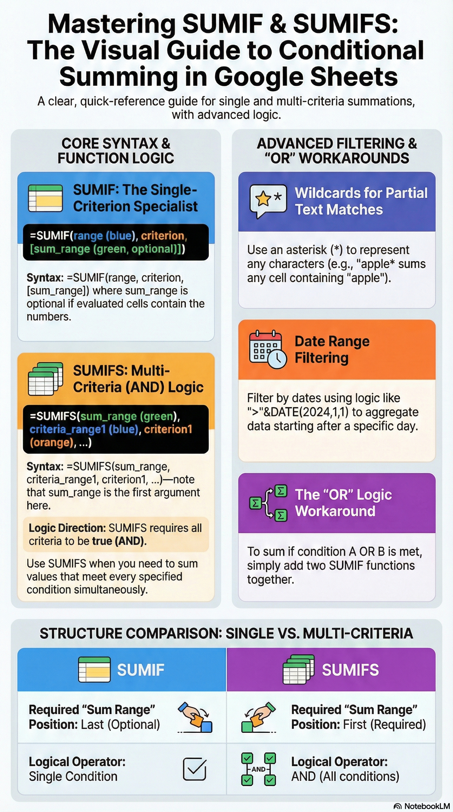
The SUMIF function adds up cell values in a range that meet a condition you specify. Here is the syntax:
=SUMIF(range, criterion, [sum_range])Let's break down each parameter:
- range — The range of cells you want to evaluate against your criterion. For example, a column of product names or category labels.
- criterion — The condition that determines which cells get summed. This can be a number, text string, cell reference, or expression like
">100". - sum_range (optional) — The range of cells to actually add up. If you omit this, Google Sheets sums the cells in
rangeitself.
A quick mental model: range is where SUMIF looks, criterion is what it looks for, and sum_range is what it adds up.
Here is a simple example. Suppose column A has department names and column B has expense amounts:
=SUMIF(A2:A20, "Marketing", B2:B20)This formula checks every cell in A2:A20. Wherever it finds "Marketing", it adds the corresponding value from B2:B20. Simple and powerful.
SUMIF Examples (Beginner to Advanced)
Let's walk through practical examples you can copy into your own sheets. Each one builds on the previous, so you will gradually see how flexible SUMIF really is.
Sum by Text Match (Exact Category)
The most common use case: sum values for a specific text label. Say you have a sales log with product categories in column A and revenue in column B.
=SUMIF(A2:A100, "Electronics", B2:B100)This returns the total revenue for all "Electronics" rows. The text match is not case-sensitive — "electronics", "ELECTRONICS", and "Electronics" all match.
You can also use comparison operators for numeric criteria:
=SUMIF(B2:B100, ">500")This sums every value in B2:B100 that is greater than 500. Notice that sum_range is omitted here, so SUMIF sums the same range it evaluates.
Sum with Wildcards (* and ?)
Wildcards are incredibly useful when your data is not perfectly standardized. Google Sheets SUMIF supports two wildcards:
- * (asterisk) — Matches any number of characters
- ? (question mark) — Matches exactly one character
For example, to sum revenue for any product containing the word "Pro":
=SUMIF(A2:A50, "*Pro*", B2:B50)This matches "MacBook Pro", "AirPods Pro", "Pro Plan", and so on. It is a lifesaver when categories or product names vary slightly across rows.
The question mark wildcard is more precise. To match any four-letter code starting with "AB" and ending with "5":
=SUMIF(A2:A50, "AB?5", B2:B50)This matches "AB15", "AB25", "ABX5" — but not "AB105" (too many characters).
If you need to search for a literal asterisk or question mark, prefix it with a tilde: ~* or ~?.
Sum by Date Range
SUMIF works well with dates, but you need to format the criterion correctly. To sum all sales on or after January 1, 2025:
=SUMIF(A2:A100, ">="&DATE(2025,1,1), B2:B100)The DATE() function ensures Google Sheets interprets the value as a proper date, avoiding locale-related issues. You can also combine two SUMIF calls to create a date range:
=SUMIF(A2:A100, ">="&DATE(2025,1,1), B2:B100) - SUMIF(A2:A100, ">="&DATE(2025,4,1), B2:B100)This gives you the total for Q1 2025 (January 1 through March 31). The first SUMIF captures everything from Jan 1 onward, and the second subtracts everything from April 1 onward.
Sum with Cell Reference as Criterion
Hard-coding criteria into formulas works for one-off calculations, but cell references make your sheets dynamic. Place your criterion in a cell (say D1), then reference it:
=SUMIF(A2:A100, D1, B2:B100)Now anyone can change the value in D1 — type "Marketing", "Sales", or "Engineering" — and the sum updates instantly. This is the foundation for building interactive dashboards in Google Sheets.
You can combine cell references with operators too:
=SUMIF(B2:B100, ">"&D1)If D1 contains 1000, this sums all values greater than 1000.
SUMIFS — Multiple Criteria Sums
When one condition is not enough, SUMIFS lets you apply two or more criteria at the same time. The syntax is slightly different from SUMIF — pay attention to the parameter order:
=SUMIFS(sum_range, criteria_range1, criterion1, criteria_range2, criterion2, ...)Notice that sum_range comes first in SUMIFS, while it comes last (and is optional) in SUMIF. This is the biggest syntax "gotcha" and the number one source of confusion between the two functions.
Here is a practical example. Sum revenue where the department is "Sales" AND the amount is greater than 500:
=SUMIFS(C2:C100, A2:A100, "Sales", C2:C100, ">500")You can stack as many criteria as you need. To add a date condition (on or after Jan 1, 2025):
=SUMIFS(C2:C100, A2:A100, "Sales", C2:C100, ">500", B2:B100, ">="&DATE(2025,1,1))All criteria use AND logic — every condition must be true for a row to be included in the sum. If you need OR logic (for example, sum where department is "Sales" OR "Marketing"), the cleanest approach is to add separate SUMIF calls:
=SUMIF(A2:A100, "Sales", C2:C100) + SUMIF(A2:A100, "Marketing", C2:C100)For datasets with many categories, the QUERY function can be a more elegant solution for OR-based aggregations.
SUMIF vs SUMIFS vs SUMPRODUCT
Choosing the right conditional sum function depends on how complex your criteria are. Here is a quick comparison:
| Feature | SUMIF | SUMIFS | SUMPRODUCT |
|---|---|---|---|
| Number of criteria | 1 | 2 or more (AND logic) | Unlimited (AND/OR) |
| OR logic support | No (need multiple calls) | No (need multiple calls) | Yes, natively |
| Wildcards | Yes (* and ?) | Yes (* and ?) | No (use SEARCH/FIND) |
| Array operations | No | No | Yes |
| Ease of use | Easiest | Easy | Advanced |
| Performance | Fast | Fast | Slower on large data |
When to use each:
- SUMIF — Single condition, simple criteria. Your go-to for everyday tasks.
- SUMIFS — Multiple AND conditions. Perfect for filtering by department AND date AND amount threshold.
- SUMPRODUCT — Complex OR logic, weighted calculations, or when you need to multiply arrays before summing. It is more powerful but harder to debug.
For most day-to-day spreadsheet work, SUMIF and SUMIFS cover 90% of conditional sum needs. Reserve SUMPRODUCT for the edge cases.
If your conditional sums are getting complicated, consider whether a pivot table might be a cleaner solution. Pivot tables handle multi-dimensional aggregation without formula complexity.
Common SUMIF Errors and Fixes
SUMIF is straightforward, but a few pitfalls trip up even experienced spreadsheet users. Here are the most common problems and how to solve them.
SUMIF Returns 0 When It Should Not
The most frequent issue. Your formula looks correct, the data is there, but SUMIF returns 0. Common causes:
- Text vs. number mismatch: If your "numbers" were imported as text (common with CSV imports), SUMIF cannot sum them. Select the column, go to Format > Number > Number to convert. If you are importing large CSV files regularly, SmoothSheet preserves data types during import so you avoid this issue from the start.
- Leading/trailing spaces: "Marketing " (with a trailing space) does not match "Marketing". Use
=SUMIF(A2:A100, TRIM(D1), B2:B100)or clean the data withTRIM()first. - Wrong range sizes: If
rangeandsum_rangehave different sizes, SUMIF only uses the dimensions ofrange. Make sure both ranges have the same number of rows.
Date Formatting Issues
Dates are notoriously tricky in spreadsheets. If your SUMIF date criterion is not working:
- Always use the DATE() function instead of text strings like "1/1/2025". Text date formats depend on your spreadsheet locale and often fail silently.
- Check date serial numbers: Select a date cell and look at the formula bar. If it shows a number (like 45658), it is a proper date. If it shows text, you need to convert it.
- Use
=DATEVALUE()to convert text dates to proper date values.
Criterion Syntax Errors
Operators must be inside quotes and concatenated with values:
- Correct:
=SUMIF(A2:A100, ">"&100) - Incorrect:
=SUMIF(A2:A100, >100)
When combining operators with cell references, use the ampersand to concatenate:
=SUMIF(A2:A100, ">="&D1, B2:B100)If you are wrapping SUMIF results in other functions and getting unexpected errors, the IFERROR function can help you handle edge cases gracefully:
=IFERROR(SUMIF(A2:A100, D1, B2:B100), 0)Performance on Large Datasets
SUMIF is efficient, but performance can degrade on sheets with hundreds of thousands of rows — especially if you have many SUMIF formulas referencing large ranges. A few tips:
- Use defined ranges (A2:A10000) instead of entire columns (A:A)
- If your source data comes from CSV or Excel files that exceed Google Sheets' performance sweet spot, use SmoothSheet's CSV Splitter to break the file into manageable chunks before importing
- Consider replacing many SUMIF calls with a single pivot table or QUERY formula
FAQ
What is the difference between SUMIF and SUMIFS in Google Sheets?
SUMIF handles a single condition, while SUMIFS supports multiple conditions with AND logic. The parameter order also differs: SUMIF puts sum_range last (and it is optional), while SUMIFS puts sum_range first. Use SUMIF for simple, single-criterion sums and SUMIFS when you need to filter by two or more conditions simultaneously.
Can SUMIF use wildcards for partial text matching?
Yes. Use * to match any number of characters and ? to match exactly one character. For example, =SUMIF(A2:A50, "*apple*", B2:B50) sums values where the corresponding cell in column A contains "apple" anywhere in the text. To search for a literal asterisk or question mark, prefix it with a tilde (~).
Why does my SUMIF formula return 0 even though there is matching data?
The most common cause is a data type mismatch — your numbers may be stored as text, especially after a CSV or Excel import. Check by selecting a cell and looking at the alignment (text aligns left, numbers align right). Convert text to numbers by selecting the range, clicking Format > Number > Number. Also check for leading or trailing spaces in text criteria using the TRIM() function.
How do I use SUMIF with dates in Google Sheets?
Use the DATE() function to build your criterion instead of typing date strings. For example: =SUMIF(A2:A100, ">="&DATE(2025,1,1), B2:B100). This avoids locale-dependent formatting issues. For a date range, subtract two SUMIF calls or use SUMIFS with both a start and end date criterion.
Conclusion
SUMIF is one of those Google Sheets functions you will use constantly once you learn it. Start with simple text matches, graduate to wildcards and date ranges, and reach for SUMIFS when a single criterion is not enough. The comparison table above should help you decide between SUMIF, SUMIFS, and SUMPRODUCT for any scenario.
The biggest gotcha? Data type mismatches from imported files. If your SUMIF returns 0 unexpectedly, check whether your numbers are actually stored as text. For teams that regularly import large CSV or Excel files into Google Sheets, SmoothSheet handles server-side processing and preserves data types — so your SUMIF formulas work correctly on the first try, without browser crashes or manual cleanup.
Got a dataset ready to crunch? Open Google Sheets, try the formulas from this guide, and see how much time conditional sums save you.