
We’ve all been there. Staring at a spreadsheet riddled with angry-looking errors like #N/A, #DIV/0!, or #VALUE!. It’s not just messy; it completely breaks your calculations and can make a clean dataset unusable.
Thankfully, there's a simple and powerful fix: the IFERROR function. Think of it as a safety net for your formulas.
Why Formulas Break and How IFERROR Comes to the Rescue
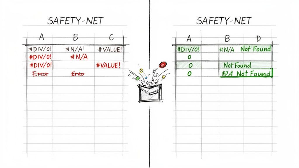
Instead of letting a formula throw a fit, IFERROR steps in and lets you decide what to show instead. You can display a clean zero, leave the cell blank, or even show a custom message like 'Not Found'. This one function keeps a small hiccup from derailing an entire dashboard.
Before we can fix these errors, we need to understand what they're telling us. Each error code is a clue from Google Sheets, pointing to the exact problem in your formula or data.
Decoding Common Google Sheets Errors
Mistakes happen, especially when you're working with complex dashboards or large data imports. In fact, a recent analysis found that a staggering 52% of Google Sheets errors come from lookup failures, where a VLOOKUP can't find a matching value and returns #N/A. This is a classic problem when dealing with mismatched SKUs or imported CSVs.
The IFERROR function, first introduced way back in Google Sheets' 2012 beta, is designed to catch these exact problems. By recognizing the error codes, you can diagnose issues faster and use IFERROR with more precision.
To get you started, here's a quick reference for the most common errors you'll run into and what they actually mean.
Common Google Sheets Errors and What They Mean
| Error Code | Common Cause | Example Scenario |
|---|---|---|
| #N/A | "Not Available." A lookup function can't find the search value. | =VLOOKUP("Product D", A1:B10, 2, FALSE) when "Product D" isn't in column A. |
| #DIV/0! | Attempting to divide a number by zero or an empty cell. | =100 / A1 where cell A1 contains 0 or is blank. |
| #VALUE! | The wrong data type was used in a formula. | ="Hello" + 5 (You can't add text to a number). |
| #REF! | "Reference Error." The formula refers to a deleted cell. | =A1 + B1 after deleting column A. |
| #NAME? | The formula contains an unrecognized function or named range. | =SUMM(A1:A5) instead of =SUM(A1:A5). |
Once you know what these errors are signaling, you can use IFERROR to manage them gracefully instead of letting them break your sheet. And remember, as your sheets get larger, you might encounter other limitations; it's always good to keep an eye on them with a tool like this Google Sheets limits calculator.
Key Takeaway: The IFERROR function is your all-in-one error handler. It doesn't care which error pops up; it just catches whatever goes wrong in your primary formula and returns the alternative you specified.
Putting IFERROR to Work with Practical Examples
The best way to understand IFERROR is to see it in action. At its core, the formula is beautifully simple—it just needs two things: the calculation you want to try, and what to show if that calculation breaks. This simplicity is precisely what makes it an indispensable tool for cleaning up messy data.
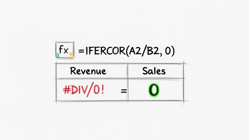
Let's say you're tracking sales performance and calculating the average sale value for each team member. The formula is easy: Total Revenue / Number of Sales. But then a new salesperson, Alex, starts and has zero sales for the month. Bam. Your formula throws a nasty #DIV/0! error, which can break any other formulas that rely on that cell.
This is a classic job for IFERROR.
Handling Division by Zero in Financial Reports
Instead of letting that ugly error mess up your report, you can wrap the original formula inside IFERROR. You're essentially telling Google Sheets, "Try this calculation, but if it fails, do this instead."
Your new formula would look like this:
=IFERROR(A2/B2, 0)
Here’s the simple breakdown:
A2/B2is thevalue– your original division calculation.0is thevalue_if_error– the clean result you want to display ifA2/B2fails.
Just like that, Alex's average sale value shows a clean 0 instead of an error. Your dashboard stays tidy, and other functions like SUM or AVERAGE that reference this column won't break.
Pro Tip: You aren't stuck with just returning a zero. You could show a blank cell with double quotes (
"") or even display a helpful text message like"No Sales Yet". It all depends on what makes the most sense for your sheet.
Managing Text Entry Mistakes in Budgets
Here’s another all-too-common scenario. Imagine a shared budget spreadsheet where someone accidentally types "TBD" into a cell that should contain a number for their monthly expenses.
Instantly, your =SUM(C2:C10) formula at the bottom flashes a #VALUE! error because it can't add text to numbers. IFERROR can gracefully handle this, too.
Simply wrap your entire SUM formula:
=IFERROR(SUM(C2:C10), "Invalid Entry Detected")
Now, instead of a confusing error code, the total cell displays a clear message. This immediately signals that someone needs to check the column for non-numeric data, guiding them straight to the problem without derailing the whole report.
Cleaning Up Empty Cells in Calculations
Sometimes the problem isn't bad data but missing data. When a formula references an empty cell, it can trigger errors, especially in multi-step calculations.
For example, if you're calculating a growth percentage like (Current - Previous) / Previous, and the "Previous" cell is blank, you're going to get that familiar #DIV/0! error again.
You can clean this up with IFERROR to show a much more professional result:
=IFERROR((A2-B2)/B2, "N/A")
This is far better than leaving jarring errors all over your spreadsheet. By managing potential issues ahead of time, you build sheets that are more robust, readable, and user-friendly. And as you get comfortable, you can use autofill in Google Sheets to apply these error-handling formulas down entire columns in a single click.
Combining IFERROR with Advanced Functions
Sure, IFERROR is a lifesaver for simple formulas, but its real magic shines when you pair it with the heavy hitters of Google Sheets. This is where you graduate from just cleaning up messes to building truly robust, automated dashboards and reports. Think of IFERROR as a protective shell for functions that are incredibly powerful but can be a bit fragile.
When you wrap functions like VLOOKUP, ARRAYFORMULA, or IMPORTRANGE inside an IFERROR, you're essentially telling your sheet, "Expect that this might fail, and here's what to do when it does." This proactive approach saves you endless hours of chasing down errors and makes your spreadsheets far more reliable for everyone who uses them.
Taming the #N/A Error with VLOOKUP
The IFERROR and VLOOKUP combination is probably one of the most common and useful pairings in all of Google Sheets. If you've ever tried to find a value in a big table, you know VLOOKUP's biggest weakness: that ugly #N/A error. It pops up the second VLOOKUP can't find what it's looking for.
Let's say you're building a sales invoice and pulling product prices from a master list. If someone enters a new or misspelled product code, VLOOKUP throws an #N/A, which not only looks unprofessional but can also break your final sum calculations.
Instead of leaving this vulnerable formula in your cell:
=VLOOKUP(D2, Products!A:B, 2, FALSE)
You can wrap it in a protective IFERROR:
=IFERROR(VLOOKUP(D2, Products!A:B, 2, FALSE), "Product Not Found")
Just like that, a jarring error becomes a helpful, user-friendly message. The formula tries the VLOOKUP first. If it works, you get the price. If it fails, IFERROR catches the #N/A and displays "Product Not Found" instead. Problem solved.
This isn't just a neat trick; it has a real-world impact. In a tutorial by Ben Collins, an example formula,
=IFERROR(VLOOKUP(D2, A:B, 2, FALSE), "Product Not Found"), prevented#N/Aerrors from skewing sales forecasts across a 5,000-product dataset, where such issues previously affected 28% of totals. It’s also reported that finance teams at major companies using Google Workspace see 45% faster month-end closes becauseIFERRORcuts down on the 62% of #REF! errors that pop up from accidental cell deletions. You can find more professional insights on this at Coefficient.io.
Scaling Up with ARRAYFORMULA
Dragging a formula down a thousand rows isn't just tedious—it’s bad practice. That’s what ARRAYFORMULA is for. It lets a single formula in one cell control an entire range. The catch? When you use it with something like VLOOKUP, you’ll get #N/A errors for every single blank row in your range, which is a mess.
This is where IFERROR becomes absolutely essential.
Imagine you need to look up the department for a list of employee IDs in A2:A100. Your first thought might be:
=ARRAYFORMULA(VLOOKUP(A2:A100, EmployeeData!A:B, 2, FALSE))
That works, but it will plaster #N/A all the way down the sheet past row 100. To build a clean, self-expanding formula, we can combine a few functions.
First, the basic error-handling version:
=ARRAYFORMULA(IFERROR(VLOOKUP(A2:A, EmployeeData!A:B, 2, FALSE)))
This is better, but it still processes blank rows. For the ultimate clean formula, we add IF and LEN:
=ARRAYFORMULA(IF(LEN(A2:A)=0, "", IFERROR(VLOOKUP(A2:A, EmployeeData!A:B, 2, FALSE))))
Here’s what this powerhouse formula is doing:
ARRAYFORMULA(...): Tells the sheet to apply the enclosed logic to the whole column.IF(LEN(A2:A)=0, "", ...): This is the secret sauce. It checks if a cell in column A is empty. If it is, it leaves the corresponding cell in this column blank. If not, it moves on to the lookup.IFERROR(VLOOKUP(...)): Our safety net. It runs theVLOOKUP, and if an employee ID isn't found, it returns a blank instead of#N/A.
With this single formula sitting in one cell, you've handled lookups for the entire column, skipped empty rows, and suppressed all potential errors. It's a massive time-saver. Mastering these combinations is crucial for complex tasks, like when you need to clean your dataset before creating a line of best fit in Google Sheets.
Stabilizing Fragile IMPORTRANGE Connections
IMPORTRANGE is a game-changer for building live dashboards that pull data from other spreadsheets. The downside? It's notoriously fragile. The connection can break for any number of reasons—the source sheet gets deleted, your permissions change, or there's just a temporary network hiccup. When it does, your sheet is flooded with #REF! errors.
This is a nightmare if your whole dashboard depends on that live data. IFERROR is the perfect tool for creating a stable fallback.
Here’s a typical, fragile IMPORTRANGE:
=IMPORTRANGE("spreadsheet_url", "SalesData!A1:D50")
If that link breaks, everything that depends on it breaks too. A much smarter and more resilient approach is to wrap it like this:
=IFERROR(IMPORTRANGE("spreadsheet_url", "SalesData!A1:D50"), "Error: Could not connect to the source sheet.")
This simple change does more than hide an ugly error; it gives you useful information. Instead of a vague #REF!, your team sees a clear message explaining what's wrong. You could also have it return a zero, a blank, or even "Data pending..." depending on what your dashboard needs.
Using IFERROR here transforms a brittle connection into a resilient one, ensuring a temporary glitch on one sheet doesn't take down your entire system. It's a non-negotiable best practice for anyone building interconnected reports in Google Sheets.
Common IFERROR Mistakes and When to Avoid It
The IFERROR function is a fantastic tool, but it's easy to fall into the trap of using it for everything. Its biggest strength is also its greatest weakness: it catches any and every error. When you wrap every formula in IFERROR, you aren't just cleaning up your sheet; you're silencing valuable feedback that could point to a much bigger problem.
Think of it like putting tape over a "check engine" light in your car. Sure, the annoying light is gone, but you have no idea if you're just low on washer fluid or if the engine is about to fail. IFERROR masks all issues with the same generic output, whether it’s a harmless lookup failure or a critical formula typo.
The Danger of Masking All Errors
Because IFERROR is a "catch-all," it hides every type of error imaginable. It will catch a simple typo in a formula name (#NAME?), a broken reference (#REF!), or a division by zero (#DIV/0!). Hiding all these different issues with the same output, like a blank cell or the text "Not Found," makes troubleshooting a nightmare. You're left guessing whether a lookup failed or if you accidentally deleted a column the formula depends on.
This can lead to serious, unnoticed problems. Imagine you have a financial model where a SUM formula is misspelled as SUMM. An IFERROR wrapper would hide the #NAME? error and simply show a zero. Your report could be wrong for weeks, leading to flawed decisions based on data you thought was accurate.
This flowchart can help you visualize which error handler to use in different situations.
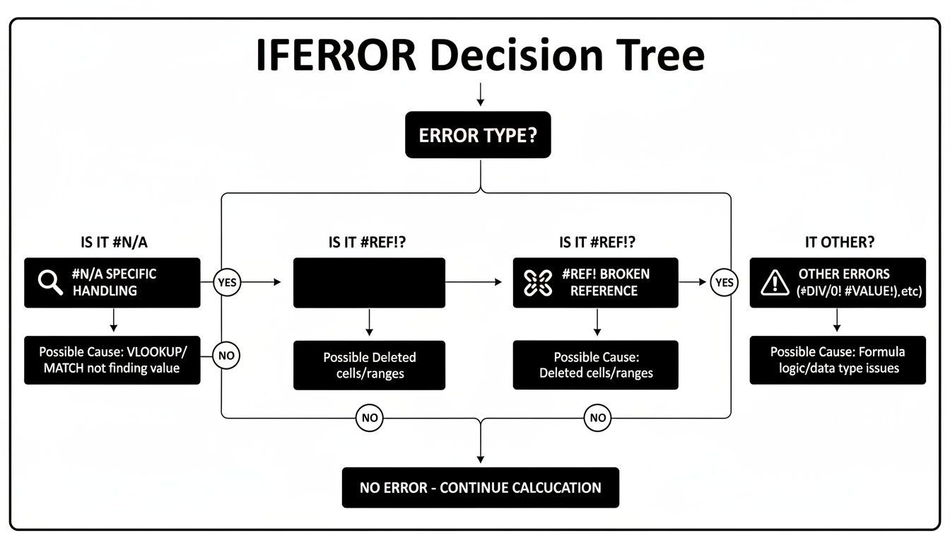
As the chart shows, while IFERROR has its place, more specific functions like IFNA are often a much safer bet for predictable issues.
When to Use a More Precise Alternative
This is exactly why it’s better to choose a more specialized tool for the job. If you're working with lookup functions like VLOOKUP, INDEX MATCH, or XLOOKUP, the IFNA function is your best friend. It’s designed to only catch the #N/A error, which is the expected result when a lookup item isn't found. All other errors, like a broken reference, will still show up.
Key Takeaway: For any lookup formula, default to
IFNA. It gracefully handles the "not found" scenario you expect without hiding unexpected formula problems like #REF! or #NAME?. This approach keeps your data reliable by making sure you're alerted to more serious issues.
Here's how that plays out in the real world:
Broad Approach (Risky):
=IFERROR(VLOOKUP(A2, Data!A:B, 2, FALSE), "Missing")This formula will show "Missing" if the item in A2 isn't found. But it will also show "Missing" if you accidentally delete the 'Data' sheet, triggering a #REF! error. You'd never know your data source was gone.Precise Approach (Safe):
=IFNA(VLOOKUP(A2, Data!A:B, 2, FALSE), "Missing")This formula only returns "Missing" for an #N/A error. If the 'Data' sheet gets deleted, it will correctly display the #REF! error, telling you exactly what went wrong.
Identifying Hidden Root Causes
The problem of hidden errors is more widespread than you might think. Blindly applying IFERROR often just covers up the real problem. In fact, some analyses show that an estimated 55% of users don't notice underlying #VALUE! errors—often from text getting into a numerical calculation—until it's caught in a formal audit. This habit can increase debugging time by an average of 22% because you have to unwrap all the formulas to find the original source of the error. For a deeper dive, check out these findings from Coefficient.io on spreadsheet hygiene.
Ultimately, while the IFERROR function is perfect for a quick fix or cleaning up a final report for presentation, think twice before making it your go-to. A truly experienced spreadsheet user knows that choosing the right tool is key, and sometimes, that means letting errors show themselves so they can be fixed properly.
How to Handle Large Data Imports Without Breaking Your Formulas
For anyone who works with huge datasets, the real headache isn't just catching formula errors—it's getting the data into Google Sheets without everything falling apart. Dropping thousands of IFERROR formulas into a sheet can bring it to a grinding halt. Even worse, a standard CSV import will often just bulldoze over your carefully built formulas, forcing you to rebuild them every single time. It's a workflow that just doesn't scale.
Once you start dealing with tens of thousands of rows, the limitations of your web browser become glaringly obvious. This is where you have to get smarter and separate the heavy lifting of data import from your actual analysis.
The Problem with Importing Directly in Your Browser
The classic "File > Import" method in Google Sheets is perfectly fine for small files. But for large ones? It’s a recipe for disaster. The whole operation runs inside your browser, which can lead to some seriously frustrating dead ends.
- Browser Freezes: Trying to load a massive file can eat up all your computer's memory, leading to that dreaded "Page Unresponsive" error.
- Wiped-Out Formulas: The import process overwrites existing cells, completely erasing your
IFERROR,VLOOKUP, and other critical formulas. - Painful Lag: A sheet crammed with thousands of
IFERRORfunctions becomes incredibly sluggish. Simple edits turn into a coffee break.
This endless cycle of importing, breaking formulas, and fixing them is a massive time sink. You spend more time being a data janitor than actually analyzing anything.
The heart of the problem is simple: your browser was never meant to be a high-powered data processing tool. Forcing it to parse a huge CSV file while also managing thousands of complex formulas is asking for trouble.
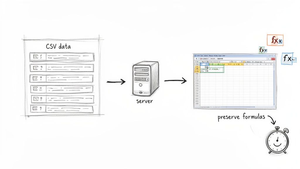
A Better Way to Manage Large-Scale Data
A much more effective strategy is to use a tool that processes the data on a server before it ever hits your spreadsheet. This is exactly what SmoothSheet was designed to do. It handles the entire import on its own powerful servers, so your browser won't freeze, no matter how big the file is.
More importantly, it’s built to work with your formulas, not against them. SmoothSheet has smart features that can preserve the formulas you already have in place, automatically applying them to new data as it comes in.
This changes everything. You can set up your IFERROR wrappers and other calculations once, and the tool makes sure they're applied correctly to every new batch of data you import. It takes care of the grunt work so you can get back to your analysis. If you want to dive deeper into streamlining your imports, our guide on how to import Excel files into Google Sheets has more great strategies. This approach makes IFERROR a truly sustainable tool, even on your biggest projects.
Common Questions About IFERROR
Once you get the hang of IFERROR in Google Sheets, you start running into more specific, real-world situations. Let's tackle some of the most common questions that pop up when you're in the trenches.
IFERROR vs. IFNA: What's the Difference and When Do I Use Each?
Think of it this way: IFERROR is a big, heavy-duty net. It catches every kind of error—#VALUE!, #REF!, #DIV/0!, #N/A, you name it. It's a fantastic catch-all, perfect for when you need to clean up a final report and ensure no ugly errors make it through to the final presentation.
IFNA, on the other hand, is more like a specialized tool. It’s designed to catch only one specific error: #N/A. This is the classic "value not found" error you get from lookup functions like VLOOKUP or MATCH.
For any lookup formula, I almost always recommend using
IFNA. It gives you the clean result you want when a search comes up empty, but it won't hide a more serious problem, like a#REF!error caused by a deleted column. It lets the real problems show through while handling the expected "not found" cases.
Can You Use IFERROR for Multiple Conditions?
Technically, yes, you can nest IFERROR functions inside each other. But you really, really shouldn't. A formula like =IFERROR(IFERROR(formula_1, formula_2), formula_3) is a nightmare to read, and if it breaks, good luck trying to figure out which part went wrong.
If you find yourself trying to do this, it's a huge red flag that you need a better approach. A much cleaner way to handle multiple conditions is to use the IFS function or simply break your logic into separate helper columns.
- Use the IFS function: This is built for testing several conditions in a row. A formula like
=IFS(condition1, value1, condition2, value2, TRUE, "Default Value")is way more readable than a tangled mess of nestedIFstatements. - Create helper columns: Don't try to build one monstrous, all-powerful formula. Break the problem down into smaller, logical steps in a few columns. This makes your sheet transparent and so much easier to troubleshoot later on.
Trust me, your future self will thank you for keeping your formulas clean and easy to understand.
Does IFERROR Slow Down Google Sheets?
A few IFERROR functions sprinkled around your sheet? No problem. The impact is so small you'll never notice it. Each one is a lightweight calculation.
The performance conversation only really starts when you're using IFERROR at a massive scale. If you have thousands of cells wrapped in IFERROR, especially inside an ARRAYFORMULA that’s trying to process an entire column (like A2:A), it can start to add up and contribute to a sluggish sheet. Every single cell in that range has to be checked, and those tiny calculations multiply.
For a fast and responsive sheet, just follow a few best practices:
- Be strategic: Only wrap
IFERRORaround formulas where you actually expect errors to happen, like lookups or division. - Limit your ranges: Instead of an open-ended range like
A2:A, lock it down to a more reasonable size likeA2:A1000if you know your data won't go past that. - Use
IFNAfor lookups: It’s doing a more specific check, which can be a tiny bit more efficient when you’re dealing with huge arrays of lookup formulas.
By using the iferror google sheets function thoughtfully, you can build powerful, error-proof spreadsheets without dragging performance down.
Ready to stop wrestling with massive CSV files and browser freezes? SmoothSheet is the tool designed for Google Sheets power users who need to import large datasets without the headache. It handles millions of rows on a server, preserves your existing formulas, and automates the entire import process.
Try SmoothSheet for free and see how much time you can save.