
If you've ever found yourself drowning in a sea of Google Sheets, constantly copy-pasting data from one file to another, then IMPORTRANGE is about to become your new best friend. It’s a powerful function that creates a live, one-way link, pulling data from a source spreadsheet directly into a destination sheet. This isn't just a simple copy; it's a dynamic connection.
What Is IMPORTRANGE and Why Should You Care?

Think of IMPORTRANGE as a data pipeline you can build between any two separate Google Sheets. Once you set it up, any changes in the source file are automatically reflected in the destination file. No more manual updates, no more version control nightmares. Just clean, consistent data.
This function is an absolute game-changer for anyone needing to centralize information. Imagine you’ve got separate sheets for regional sales, another for project timelines, and a third for inventory. IMPORTRANGE lets you pull the most important metrics from all of them into one master dashboard.
It's perfect for things like:
- Centralized Reporting: Combining data from different teams into a single, comprehensive view.
- Data Security: Sharing just a specific chunk of data with someone without giving them access to your entire sensitive source file.
- Automated Workflows: Building reports that update themselves, freeing you up from soul-crushing repetitive tasks.
Back around 2018, when Google Sheets really started taking off in the business world, IMPORTRANGE quickly became a go-to tool for anyone juggling multiple data sources. It’s been a cornerstone function ever since.
The Basic Formula Structure
Getting started with the formula is surprisingly simple. It only needs two pieces of information, which we call arguments.
=IMPORTRANGE("spreadsheet_url", "range_string")
spreadsheet_url: This is the full web address of the Google Sheet you want to pull data from. Just copy it from your browser's address bar. Pro tip: you can also just use the long spreadsheet ID from the URL to keep your formula a bit cleaner.range_string: This tells the function exactly which cells to import. You have to include the sheet (or tab) name, an exclamation mark, and the cell range. For example,"Sales!A1:D50".
Granting Access: A Crucial First Step
The very first time you connect to a new spreadsheet with IMPORTRANGE, you'll see a big, scary #REF! error. Don't panic! This isn't a mistake; it's a security feature. Google needs you to explicitly approve the connection between the two sheets.
To fix it, just hover your mouse over the cell with the formula. A small blue button that says "Allow access" will pop up. Click it, and your data will appear. You only have to do this once for each new source sheet you link to.
This one-time handshake trips up a lot of new users, but it's an essential step to make sure you control who sees your data. After mastering this, you might be interested in our guide on how to import Excel into Google Sheets, which tackles similar data migration challenges.
Putting IMPORTRANGE to Work in the Real World
Knowing the syntax is great, but the real magic of IMPORTRANGE happens when you see it solve actual business problems. Let's move past the theory and look at a few everyday situations where this function can genuinely save you hours of mind-numbing work and make your data far more reliable.
These are the kinds of setups that turn a simple spreadsheet into a powerful, automated reporting tool.
Centralizing a Master Product List
Here’s a classic scenario: managing a master product list. Your company probably has a single Google Sheet that acts as the "source of truth" for all product IDs, names, prices, and inventory levels. It’s critical information.
The sales and marketing teams need this data for their own work, but you can't just give everyone editor access to your master file. That's a recipe for disaster.
Instead of emailing outdated copies, you can use IMPORTRANGE to safely pipe that data directly into their departmental sheets. For example, the inventory team could drop this formula into their own sheet:
=IMPORTRANGE("spreadsheet_url_of_master_list", "Products!A2:E500")
This creates a live, read-only mirror of the official product list. Now, when a product manager updates a price in the master sheet, the change instantly appears in the inventory team's sheet. No more data mix-ups, and everyone is guaranteed to be working with the latest info.
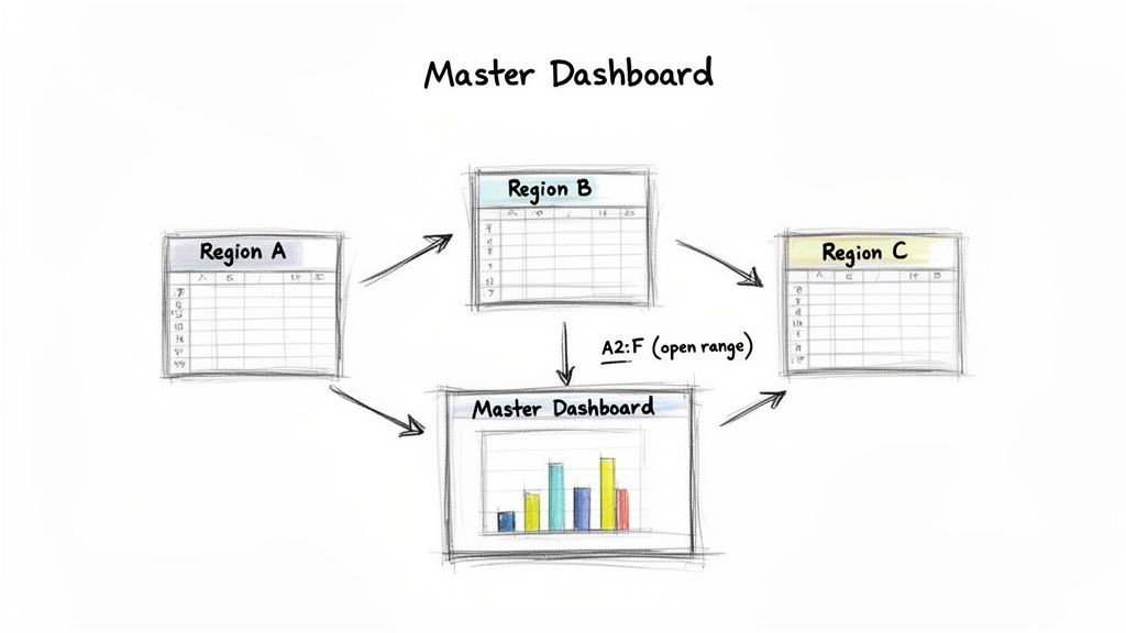
Consolidating Regional Sales Data
Another fantastic use case is building a unified dashboard from separate reports. Imagine your company has three sales regions—North, South, and West—and each team tracks their numbers in their own Google Sheet. The sales director, of course, needs one place to see the big picture.
This is where stacking IMPORTRANGE formulas with curly braces {} is a game-changer. It’s a technique for pulling data from multiple sources and neatly stacking them into a single, continuous list.
Pro Tip: When stacking data this way, you only want the header row from your first sheet. For all the other
IMPORTRANGEfunctions, make sure your range starts from row 2 (likeA2:F). This little trick prevents you from getting repeated headers cluttering up your combined dataset.
The formula in the master dashboard would look something like this:
={IMPORTRANGE("north_sales_url", "SalesData!A1:F"); IMPORTRANGE("south_sales_url", "SalesData!A2:F"); IMPORTRANGE("west_sales_url", "SalesData!A2:F")}
Let's quickly break down what this powerful one-liner is doing:
- The curly braces
{...}create a virtual array, telling Sheets to combine the results of the formulas inside. - The first
IMPORTRANGEpulls the complete dataset from the North region, headers and all (A1:F). - The semicolon
;is the key here. It’s a stacking operator that tells the formula to place the next chunk of data directly underneath the previous one. - The next two
IMPORTRANGEcalls pull data from the South and West sheets, but they cleverly start from row 2 (A2:F) to skip the redundant headers.
Just like that, you’ve built a comprehensive, self-updating sales report. As the regional teams add new sales, the main dashboard automatically grows, giving a real-time view of company performance without any manual copy-pasting.
For those in finance facing similar consolidation headaches, our guide on how finance teams import Excel to Google Sheets offers more tailored strategies. These examples show IMPORTRANGE is more than just a function—it's a core building block for creating automated and trustworthy data systems in Google Sheets.
Combine IMPORTRANGE with QUERY for Smarter Reports
Using IMPORTRANGE by itself is a bit like opening a firehose. It's powerful, sure, but it dumps everything from the source sheet into your new one, whether you need it or not. The real magic happens when you pair it with the QUERY function. Think of this combo as adding a smart nozzle to that firehose, letting you control exactly what data comes through and how it's shaped.
By wrapping IMPORTRANGE inside a QUERY, you can tell Google Sheets to filter, sort, and select specific columns before that data ever hits your sheet. This is a game-changer for performance. You're no longer importing a massive dataset just to hide most of it; you're creating a lean, targeted, and much faster report from the get-go.
The Basic Setup: QUERY + IMPORTRANGE
The fundamental idea is simple: IMPORTRANGE fetches the data, and QUERY immediately steps in to process it. The structure looks like this:
=QUERY(IMPORTRANGE("spreadsheet_url", "range_string"), "query_statement")
Now, here’s the one thing that trips everyone up at first. When you use QUERY with IMPORTRANGE, you can’t refer to columns by their letters (like A, B, C). Instead, you have to use a special notation: Col1, Col2, Col3, and so on.
Col1 is always the first column of your imported range, Col2 is the second, and so on, no matter what their original letters were.
So, if your IMPORTRANGE is pulling D:G from the source sheet:
Col1refers to column DCol2refers to column ECol3refers to column FCol4refers to column G
Nailing this Col syntax is the secret to making this powerhouse combination work.
Filtering Data Before It Arrives
Let's say you have a master sales sheet with data from all four quarters. You just need to build a report for Q4. Bringing over all the data would be a massive waste of resources and will absolutely slow your sheet down.
Here’s how you’d pull only the sales data for "Q4," assuming the quarter is listed in the 5th column of your source range (E):
=QUERY(IMPORTRANGE("source_sheet_url", "SalesData!A:G"), "SELECT * WHERE Col5 = 'Q4'")
Let's quickly break that down.
- The
IMPORTRANGEpart grabs the entire block of data from columns A through G. - The
QUERYthen takes that data and applies a filter:SELECT *says "give me all the columns," but theWHERE Col5 = 'Q4'part only keeps the rows where the fifth column is exactly 'Q4'.
This is so much more efficient than importing thousands of rows you’re just going to ignore.
When you nest functions like this, you're telling Google's servers to do the heavy lifting of filtering the data before the final, clean results are sent to your sheet. This dramatically cuts down on lag and keeps your spreadsheet feeling snappy.
Creating Highly Specific, Polished Reports
You can get even more sophisticated. What if you need a report of your top Q4 sales, but you only want to see the product name (column B), the sale date (column D), and the final sale amount (column G)? And you want it sorted from the highest sale to the lowest.
Easy. Your formula just gets a little more specific:
=QUERY(IMPORTRANGE("source_sheet_url", "SalesData!A:G"), "SELECT Col2, Col4, Col7 WHERE Col5 = 'Q4' ORDER BY Col7 DESC")
Here, we've added a couple of new commands to the query string:
SELECT Col2, Col4, Col7: This tellsQUERYto cherry-pick only the 2nd, 4th, and 7th columns, leaving the rest behind.ORDER BY Col7 DESC: This sorts the final results by the 7th column (the sale amount) in descending order (DESC), putting your biggest wins right at the top.
With just one formula, you've built a live, self-updating report that's perfectly filtered and formatted. For more advanced tricks, I highly recommend diving into our guide to the Google Sheets QUERY function.
This isn't just a neat trick; it's a standard practice for anyone serious about Google Sheets. In fact, a 2023 industry analysis found that about 75% of data analysts were regularly using this IMPORTRANGE and QUERY combo for their dynamic reports. It’s a testament to just how effective it is. You can also explore more powerful spreadsheet formulas on benlcollins.com.
How to Fix Common IMPORTRANGE Errors
Sooner or later, every IMPORTRANGE user gets initiated into the club by seeing a formula error. It’s practically a rite of passage. But don't sweat it—these errors are almost always caused by a few common, fixable issues. Think of this as your troubleshooting field guide.
When an error pops up, the key is not to panic. Instead, just systematically check the most likely culprits. A single misplaced character or a forgotten permission step is often all that stands between you and your data.
Decoding the #REF! Error
The #REF! error is, by far, the most frequent one you'll run into. It’s a general-purpose error that can mean a few different things, but it's usually one of two main problems.
First, and most common for new connections, is a permission issue. IMPORTRANGE requires you to explicitly grant access for one sheet to pull data from another. If you see #REF!, hover your cursor over the cell. A blue "Allow access" button should appear. Clicking this establishes the connection and, nine times out of ten, solves the problem instantly.
If that button doesn't show up or doesn't fix it, your next move is to meticulously check your formula's syntax.
- Is the URL correct? Double-check the
spreadsheet_url. Even one wrong character in the spreadsheet ID will break the connection. - Is the range string accurate? Look closely at the sheet name and cell range. A simple typo like
"Sales Data!A:F"instead of"Sales!A:F"is an easy mistake to make. - Does the range even exist? Make sure the range you specified (e.g.,
A1:Z1000) is actually present in the source sheet.
The
#REF!error can also pop up if your formula is trying to paste data into cells that already contain something else. Google Sheets needs a completely empty space for the imported data and will throw this error if it can't overwrite existing content.
Other Common Culprits like #N/A and #VALUE!
While #REF! is the star of the show, other errors like #N/A, #VALUE!, and the dreaded infinite "Loading..." state can also make an appearance. Each one points to a different kind of problem.
A #N/A error usually means "not available." You’ll often see this when you've paired IMPORTRANGE with a lookup function like VLOOKUP. It’s telling you that the lookup value wasn't found in the imported data, not that the import itself failed.
The #VALUE! error, on the other hand, frequently signals a syntax problem. This is especially true when you're combining multiple IMPORTRANGE functions with curly braces {}. This error often means the ranges you're trying to stack on top of each other don't have the same number of columns, which is a must for creating a valid array.
And if your sheet just gets stuck on "Loading...", you're likely pushing the function's limits. This can happen if you're importing way too much data or creating long, chained dependencies where one import relies on another.
This decision tree helps visualize when it's better to filter data with QUERY to avoid those performance headaches.
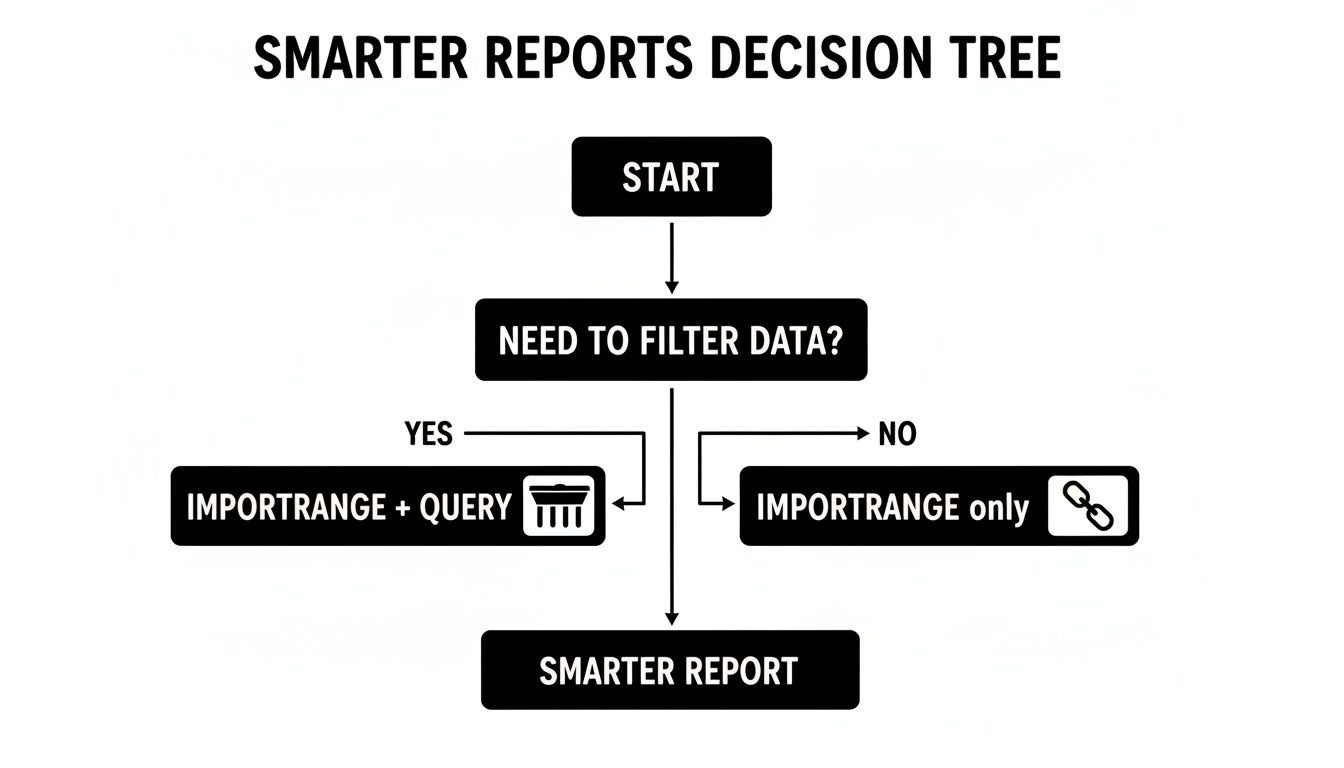
As you can see, if you need to bring in only specific data, combining IMPORTRANGE with QUERY is the smarter choice for better performance and more targeted reports.
Here’s a quick-reference table to help you diagnose and fix these common hiccups.
Common IMPORTRANGE Error Fixes
| Error Code | Common Cause | How to Fix |
|---|---|---|
| #REF! | Permission Not Granted: The destination sheet hasn't been authorized to pull data. | Hover over the cell and click the "Allow access" button that appears. |
| #REF! | Incorrect URL/Range: The spreadsheet URL or the sheet/cell reference is wrong. | Carefully check for typos in both the URL and the range string (e.g., "Sheet1!A:B"). |
| #REF! | Output Range Blocked: The cells where the data should go are not empty. | Clear out all data from the cells where the formula is trying to output its results. |
| #N/A | Lookup Value Not Found: Often seen when combined with functions like VLOOKUP or MATCH. |
The import is working, but your lookup function can't find the specified value. Check your search key. |
| #VALUE! | Mismatched Columns: Usually happens when stacking multiple imports with {} and they don't have the same column count. |
Ensure all vertically stacked IMPORTRANGE functions import the exact same number of columns. |
| "Loading..." | Overloaded Formula: Importing too much data or chaining too many IMPORTRANGE functions together. |
Reduce the amount of data being imported. Try wrapping it in a QUERY to filter the data at the source. |
With a little practice, you'll be able to spot these issues in seconds.
Managing Permissions and Data Security
Fixing technical errors is one thing, but there's a serious data governance side to IMPORTRANGE that many people miss. Once you grant access, you create a permanent, invisible link.
The big challenge here is that Google provides no built-in dashboard to see which spreadsheets are pulling data from your source sheet. This creates a massive blind spot. In fact, some data security audits have flagged this as a real concern, with one study noting that 44% of shared corporate sheets had active IMPORTRANGE connections from unknown or unauthorized destination sheets. You can dig into these privacy implications for Google Sheets on Google's support forum.
To keep your data safe, here are a few best practices I always follow:
- Create "Viewer" Only Sheets: When possible, I create dedicated, view-only versions of sensitive data sheets just for importing. This prevents the destination user from ever accessing the original.
- Be Strict with Sharing: I'm extremely careful about who I share source sheets with. Remember, anyone with "View" access can pull its data into another sheet.
- Audit Access Regularly: Every so often, I review the sharing settings on my most important spreadsheets and remove anyone who no longer needs access. It's simple but effective hygiene.
Handling Large Datasets and Performance Issues
IMPORTRANGE is an amazing tool for connecting reports and building dashboards, but it definitely has a breaking point. Once you start pulling in tens of thousands of rows or creating complex chains of imports, you’ll quickly run into its performance limits.

To fix the slowdown, you first have to understand why it’s happening. The IMPORTRANGE function is client-side, which is a technical way of saying it downloads the entire source range directly into your browser every single time your sheet recalculates. This eats up a ton of your computer’s memory and processing power.
Why Your Sheet Is Crawling
Pulling in a small range like A1:D100 is no big deal. But try to import a whole tab (A:Z) from a sheet with 50,000 rows, and your browser is suddenly tasked with downloading and crunching a massive amount of data. This is what leads to that dreaded "Page Unresponsive" error, forcing you to kill the tab and start over.
The problem gets way worse when you start chaining imports together. Think of it like a domino effect:
- Sheet A holds your raw data.
- Sheet B uses
IMPORTRANGEto pull from Sheet A. - Sheet C then uses
IMPORTRANGEto pull the processed data from Sheet B.
Before Sheet C can load, it has to wait for Sheet B to finish its own import from Sheet A. This creates a cascade of delays where each link in the chain adds another layer of processing and another potential point of failure.
Every
IMPORTRANGEis a heavy request to Google's servers. The more you add, the more you're asking your browser to handle, which directly causes lag, slow loading, and a genuinely frustrating experience.
Practical Limits and What to Expect
While Google’s official docs mention a 10MB data limit, I’ve found that you’ll feel the pain long before you hit any official error. From my experience and what I've seen in the community, performance issues really start to creep in when you approach these thresholds:
- Cell Count: Importing more than 50,000 cells in a single function often leads to noticeable lag.
- Chained Imports: Relying on more than two or three "levels" of chained imports is just asking for an unstable sheet.
- Formula Density: Sprinkling dozens of separate
IMPORTRANGEformulas across one sheet will absolutely cripple it.
The best way to handle this is to consolidate your imports. Instead of ten formulas pulling ten small ranges, use one IMPORTRANGE to pull a single, large block of data into a dedicated "Data Import" tab. Then, use simple, local cell references throughout your sheet to work with that data. This approach makes just one external call, which dramatically speeds things up.
When You've Outgrown IMPORTRANGE
If you’re constantly hitting these limits and watching your browser freeze, it’s a clear signal you’ve pushed IMPORTRANGE beyond its intended use. At that scale, you need a more robust, server-side solution that does the heavy lifting for you, completely outside of your browser.
This is where specialized tools come into the picture. A server-side importer processes data on a powerful external server and then gently places the final, clean results into your Google Sheet. This completely sidesteps the browser-based limitations that cause IMPORTRANGE to choke on large files. If this sounds like a familiar struggle, our guide on how to upload large CSV files to Google Sheets without browser crashes walks through a much more scalable approach.
When your data needs get serious, it's time to consider these alternatives:
| Method | Best For | How It Works |
|---|---|---|
IMPORTRANGE |
Small to medium datasets and simple dashboards. | A client-side function that downloads data directly to your browser. |
| Google Apps Script | Custom, scheduled data pulls with moderate data sizes. | Server-side JavaScript that you can schedule to run automatically. |
| Third-Party Tools | Massive datasets (hundreds of thousands of rows or more). | Secure, dedicated servers handle the entire import process for you. |
Ultimately, knowing the limitations of IMPORTRANGE is just as important as knowing how to use it. It's a fantastic function for many scenarios, but for any heavy-duty data work, switching to a server-side solution will save you countless hours of frustration and keep your spreadsheets running smoothly.
Common IMPORTRANGE Questions Answered
Even after you get the hang of IMPORTRANGE, a few questions tend to pop up again and again. I've heard them all over the years, so let's walk through the most common ones to get you past any sticking points.
Can I Import Cell Formatting, Too?
This is probably the number one question I get. The short answer is no, IMPORTRANGE only pulls in the raw cell values. It’s completely blind to any formatting you’ve applied.
That means all your beautiful colors, bold text, currency symbols, and conditional formatting rules get left behind. You’ll have to reapply any of that styling in the new sheet once the data is there.
How Often Does the Data Actually Refresh?
Google's official line is that updates can take up to five minutes to appear. From my experience, it's usually much quicker than that—often just a matter of seconds.
But it’s definitely not instant. If you’re staring at your sheet waiting for a critical update, you can try to give it a nudge:
- Refresh the page: A simple CTRL+R or CMD+R can force the sheet to recalculate.
- Re-open the sheet: Sometimes closing the tab and opening it again does the trick.
The key is to remember IMPORTRANGE works on its own schedule. It’s built for keeping things generally in sync, not for split-second, real-time dashboards.
My Take: Don't rely on
IMPORTRANGEfor time-critical reports where a few minutes of delay could cause problems. It’s designed for convenience, not instant updates.
Is There a Limit on How Many IMPORTRANGE Functions I Can Use?
There's no official, hard-coded limit, but there is absolutely a practical one. Every single IMPORTRANGE function you add is another data call your spreadsheet has to make over the internet.
Start adding dozens of them, and you'll feel the pain. Your sheet will start to load slowly, calculations will lag, and you might even see those frustrating "Loading..." messages.
The best way to handle this is to import smarter, not harder. Instead of pulling ten different little ranges with ten separate formulas, use one single IMPORTRANGE to pull a larger, consolidated block of data into a hidden "Import" tab. Then, use formulas to reference that local data throughout the rest of your workbook. It's way more efficient.
I Already Granted Access, So Why Am I Still Seeing a #REF! Error?
Ah, the classic. You hit the "Allow access" button, but the #REF! error just sits there, mocking you. When this happens, the problem is almost always a simple typo in your range_string.
Permission is just the first hurdle. After that, you have to get the syntax perfect. Go back and check these common culprits:
- Sheet Name Typos: Is the sheet name exactly right, including spaces?
"Sheet1"is not the same as"Sheet 1". - Non-existent Range: Did you ask for
A1:Z5000when the source sheet only has 1000 rows? The range must exist. - The Missing Exclamation Mark: You absolutely need that
!between the sheet name and the cell range, like"Dashboard Data!A1:G50".
Nine times out of ten, fixing one of these small details will clear up that stubborn #REF! error right away.
When IMPORTRANGE just can't handle your massive datasets, your browser will grind to a halt. SmoothSheet gets around this by processing the import on powerful servers instead of your computer. You can upload huge CSV or Excel files directly into Google Sheets without ever worrying about freezes or row limits. Learn how SmoothSheet can make your large data imports fast and reliable.