Google Sheets QUERY Function: SQL for Your Spreadsheet

The Google Sheets QUERY function is the closest thing you will get to writing SQL without leaving your spreadsheet. If you have ever wished you could run database-style queries on your data -- filtering rows, grouping results, sorting columns -- QUERY does exactly that with a single formula.

Whether you are analyzing sales figures, cleaning imported CSV data, or building dynamic reports, QUERY handles it all. It uses Google Visualization API Query Language, which borrows heavily from SQL syntax. Once you learn the basics, you will wonder how you ever managed without it.

In this guide, I will walk you through the complete QUERY function syntax, every essential clause with real examples, advanced techniques like dynamic cell references and cross-sheet queries, and the common errors that trip up even experienced users.

Key Takeaways:QUERY is the most powerful built-in function in Google Sheets -- SQL-like queries on spreadsheet dataThe syntax follows a strict clause order: SELECT, WHERE, GROUP BY, PIVOT, ORDER BY, LIMIT, OFFSET, LABEL, FORMATDate handling is the #1 source of QUERY errors -- always use date 'yyyy-mm-dd' formatMixed data types cause silent data loss -- QUERY treats the minority type as nullFor large datasets, SmoothSheet imports CSV/Excel files into Google Sheets without browser crashes, so QUERY can analyze them

What Is the QUERY Function?

The QUERY function lets you run SQL-like queries directly on your Google Sheets data. Think of it as a mini database engine built right into your spreadsheet. You write a query string that tells Sheets exactly what data you want, how to filter it, and how to present the results.

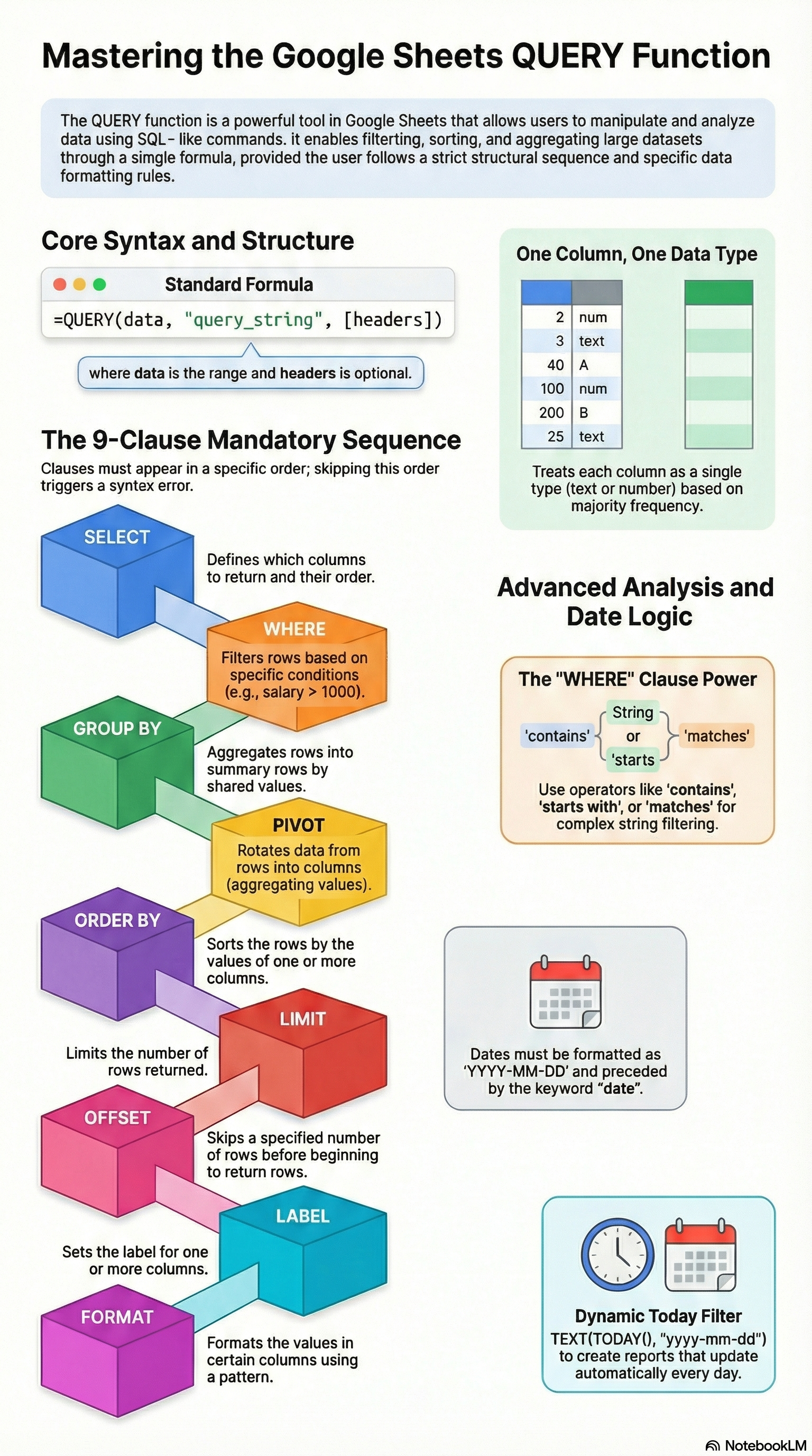
Here is the basic syntax:

=QUERY(data, query, [headers])

It works by taking a range of cells, applying your query conditions, and returning a filtered, sorted, or aggregated result set -- all in a single formula. Unlike INDEX MATCH or XLOOKUP, which look up individual values, QUERY can return entire tables of results at once.

Why It Is Like SQL for Spreadsheets

QUERY uses the Google Visualization API Query Language, which mirrors SQL syntax closely. If you have ever written SELECT * FROM table WHERE column > 100, you already know the basics. The main difference? Instead of table names, you reference cell ranges. Instead of column names, you use column letters (A, B, C) or Col1, Col2 for arrays.

When to Use QUERY vs. FILTER or VLOOKUP

Use QUERY when you need to:

• Aggregate data -- SUM, COUNT, AVG, MAX, MIN by groups (FILTER cannot do this)
• Sort and limit results -- get the top 10 rows by sales amount
• Rename output headers -- clean up column names in your results
• Combine multiple operations -- filter, sort, group, and relabel in one formula

Use FILTER for simple row filtering. Use VLOOKUP or XLOOKUP for single-value lookups. QUERY is the right choice when your analysis needs more than one operation at a time.

QUERY Function Syntax Explained

Let us break down each parameter so you know exactly what goes where.

The Data Parameter

The first argument is the range of cells you want to query. This can be a simple range like A1:E100, a full column reference like A:E, a named range, or even an array created with curly braces {}.

Important: When your data range is an array (built with {}, returned by IMPORTRANGE, or combined from multiple tabs), you must reference columns as Col1, Col2, Col3 instead of letter-based references like A, B, C. This is one of the most common sources of confusion.

The Query String (Google Visualization API Query Language)

The second argument is where the magic happens. This is a text string containing your SQL-like commands. It must be enclosed in double quotes:

=QUERY(A1:E100, "SELECT A, B WHERE C > 100 ORDER BY B DESC", 1)

The clauses within the query string must follow a specific order. If you mix them up, the formula returns an error. The correct order is: SELECT, WHERE, GROUP BY, PIVOT, ORDER BY, LIMIT, OFFSET, LABEL, FORMAT, OPTIONS.

The Headers Parameter

The third argument is optional but recommended. It tells QUERY how many header rows exist at the top of your data range:

• 1 -- your data has one header row (most common)
• 0 -- your data has no headers; treat the first row as data
• -1 or omitted -- Google Sheets guesses the number of header rows

Pro tip: Always specify the headers parameter explicitly. Letting Sheets guess can lead to unexpected behavior, especially when your header text looks like data values.

Essential QUERY Clauses with Examples

Let us walk through the most commonly used clauses. For all examples, imagine a dataset in A1:E20 with columns: Name (A), Region (B), Date (C), Sales (D), Product (E).

SELECT -- Choose Specific Columns

SELECT determines which columns appear in your output and in what order. If you omit SELECT, all columns are returned.

=QUERY(A1:E20, "SELECT A, B, D", 1)

This returns only the Name, Region, and Sales columns. You can also select all columns with:

=QUERY(A1:E20, "SELECT *", 1)

WHERE -- Filter Rows by Condition

WHERE filters your data to only include rows that match specific conditions.

=QUERY(A1:E20, "SELECT * WHERE D > 1000", 1)

For text comparisons, wrap the value in single quotes:

=QUERY(A1:E20, "SELECT * WHERE B = 'West'", 1)

You can also filter for non-empty cells:

=QUERY(A1:E20, "SELECT * WHERE A IS NOT NULL", 1)

ORDER BY -- Sort Results

ORDER BY sorts your output by one or more columns, ascending (ASC) or descending (DESC).

=QUERY(A1:E20, "SELECT * ORDER BY D DESC", 1)

Sort by multiple columns:

=QUERY(A1:E20, "SELECT * ORDER BY B ASC, D DESC", 1)

GROUP BY -- Aggregate Data (SUM, COUNT, AVG)

GROUP BY lets you aggregate values, similar to SQL. Use it with functions like SUM, COUNT, AVG, MAX, and MIN.

=QUERY(A1:E20, "SELECT B, SUM(D) GROUP BY B", 1)

This totals Sales by Region. You can count items per category too:

=QUERY(A1:E20, "SELECT E, COUNT(A) GROUP BY E", 1)

LIMIT -- Return Only N Rows

LIMIT restricts how many rows the query returns. It works great with ORDER BY to get "top N" results:

=QUERY(A1:E20, "SELECT A, D ORDER BY D DESC LIMIT 5", 1)

This returns the top 5 salespeople by amount. You can also skip rows with OFFSET:

=QUERY(A1:E20, "SELECT * LIMIT 5 OFFSET 10", 1)

LABEL -- Rename Column Headers

LABEL renames the column headers in your output. This is especially useful after aggregation, where headers default to things like "sum Sales":

=QUERY(A1:E20, "SELECT B, SUM(D) GROUP BY B LABEL B 'Region', SUM(D) 'Total Sales'", 1)

Now your output shows clean "Region" and "Total Sales" headers instead of the default names.

Advanced QUERY Techniques

Once you have the basics down, these techniques will take your QUERY skills to the next level.

Multiple Conditions (AND, OR)

Combine conditions in the WHERE clause using AND and OR. Use parentheses to group logic:

=QUERY(A1:E20, "SELECT A, B, D WHERE (B = 'West' AND D > 1000) OR B = 'East'", 1)

For date range filtering:

=QUERY(A1:E20, "SELECT * WHERE C >= date '2025-01-01' AND C <= date '2025-12-31'", 1)

QUERY with Cell References (Dynamic Queries)

Hard-coding values works for one-off queries, but dynamic queries let you build interactive dashboards. The syntax differs depending on the data type in your reference cell:

For numbers -- no single quotes needed:

=QUERY(A1:E20, "SELECT * WHERE D > " & G1, 1)

For text strings -- wrap in single quotes:

=QUERY(A1:E20, "SELECT * WHERE B = '" & G1 & "'" , 1)

For dates -- use the date keyword with TEXT conversion:

=QUERY(A1:E20, "SELECT * WHERE C > date '" & TEXT(G1, "yyyy-mm-dd") & "'" , 1)

Pair these with IFERROR to handle cases where the reference cell is empty, preventing ugly error messages in your dashboard.

QUERY Across Sheets (Combine with IMPORTRANGE)

To query data from a different Google Sheets file, nest IMPORTRANGE inside QUERY. Remember: you must use Col1, Col2 notation instead of column letters when querying imported data:

=QUERY(IMPORTRANGE("spreadsheet_url", "Sheet1!A1:E"), "SELECT Col1, Col3 WHERE Col2 = 'North'", 1)

You will need to authorize the connection between sheets the first time. For more details on pulling data between spreadsheets, check out our complete IMPORTRANGE guide.

If you are importing large CSV or Excel files to query across multiple sheets, SmoothSheet handles the heavy lifting -- it processes files server-side so your browser does not crash, even with datasets in the hundreds of thousands of rows.

Nested QUERY Functions

You can use the result of one QUERY as the data source for another. This is the workaround for Google Sheets lacking a HAVING clause (which filters after aggregation in SQL):

=QUERY(QUERY(A1:E20, "SELECT E, COUNT(A) GROUP BY E", 1), "SELECT * WHERE Col2 > 5", 1)

The inner query groups products and counts them. The outer query filters to show only products with more than 5 sales. Notice the outer query uses Col2 because it is querying an array result, not a direct cell range.

Common QUERY Errors and Fixes

QUERY is powerful, but it has some quirks that catch even experienced spreadsheet users off guard. Here are the most common problems and their solutions.

#VALUE! Error (Column Type Mismatch)

A #VALUE! error usually means your query string has a syntax problem. The most common causes:

• Wrong clause order: The clauses must appear in this exact order: SELECT, WHERE, GROUP BY, PIVOT, ORDER BY, LIMIT, OFFSET, LABEL, FORMAT. Swap any two and you get an error.
• Cell reference syntax: When concatenating cell references, numbers do not need single quotes but text strings do. Missing or extra quotes break the formula.
• Column letter case: Column identifiers must be uppercase. "SELECT a" fails; "SELECT A" works.

Date Handling in QUERY

Dates are the single biggest source of QUERY headaches. Google Sheets stores dates as serial numbers internally, but the QUERY language needs them as formatted string literals.

The wrong way (causes #VALUE! error):

=QUERY(A1:E20, "SELECT * WHERE C > 1/1/2025", 1)  // WRONG

Also wrong (date format not recognized):

=QUERY(A1:E20, "SELECT * WHERE C > date '01/15/2025'", 1)  // WRONG

The correct way -- use the date keyword with yyyy-mm-dd format:

=QUERY(A1:E20, "SELECT * WHERE C > date '2025-01-01'", 1)  // CORRECT

With a cell reference:

=QUERY(A1:E20, "SELECT * WHERE C > date '" & TEXT(G1, "yyyy-mm-dd") & "'" , 1)

With today's date:

=QUERY(A1:E20, "SELECT * WHERE C > date '" & TEXT(TODAY(), "yyyy-mm-dd") & "'" , 1)

Always use the date keyword, always use yyyy-mm-dd format, and always wrap dates in single quotes inside the query string.

Mixed Data Types Problem

This is QUERY's sneakiest issue. When a column contains mixed data types (for example, mostly numbers but some text entries like "N/A" or "TBA"), QUERY determines the column type by majority. The minority type values are silently treated as null -- they simply disappear from your results without any error message.

For example, if column D has 80% numbers and 20% text entries, QUERY treats column D as numeric and those text entries become empty cells in the output.

Fix: Force the column to text before querying

=ARRAYFORMULA(QUERY({A1:A, TO_TEXT(D1:D)}, "SELECT Col1, Col2 WHERE Col2 IS NOT NULL", 1))

By wrapping the problematic column in TO_TEXT(), all values become strings and nothing disappears. Note that you switch to Col1, Col2 notation when using an array.

This is especially common when importing CSV data into Google Sheets. If your import contains mixed-type columns, consider using SmoothSheet's CSV Validator to identify and fix data type inconsistencies before importing.

Headers Showing as "Column1, Column2"

If your output headers show generic labels like "Column1" or "sum Sales" instead of your actual column names, here are the fixes:

• Set the headers parameter: Make sure the third argument in your QUERY matches your data. Use 1 if your range includes one header row.
• Use LABEL: After aggregation functions, headers change. Use LABEL SUM(D) 'Total Sales' to rename them.
• Array sources: When querying arrays (from {} or IMPORTRANGE), original headers may not carry over. LABEL is your best friend here.

Frequently Asked Questions

How Do I Use the QUERY Function in Google Sheets?

Type =QUERY(data_range, "query_string", headers) in any cell. The data range is your source data, the query string contains SQL-like clauses (SELECT, WHERE, ORDER BY, etc.), and headers tells the function how many header rows exist. For example: =QUERY(A1:D100, "SELECT A, B WHERE C > 50 ORDER BY D DESC", 1). The function returns a filtered, sorted result set directly in your sheet.

Can QUERY Replace VLOOKUP?

For many use cases, yes. QUERY can do everything VLOOKUP does -- and more. Where VLOOKUP returns a single value from one column, QUERY can return multiple columns and multiple rows at once. It also does not require your lookup column to be the leftmost column (a classic VLOOKUP limitation). However, for simple single-value lookups, XLOOKUP or INDEX MATCH may be simpler to write and easier to maintain.

How Do I Use QUERY with Multiple Conditions?

Use AND and OR in the WHERE clause to combine conditions. For example: "SELECT * WHERE B = 'West' AND D > 1000" returns rows where the region is West and sales exceed 1,000. Use parentheses to group logic when mixing AND and OR: "SELECT * WHERE (B = 'West' AND D > 1000) OR B = 'East'".

Does QUERY Work with IMPORTRANGE?

Yes. Nest IMPORTRANGE inside QUERY to query data from another Google Sheets file: =QUERY(IMPORTRANGE("url", "Sheet1!A:E"), "SELECT Col1 WHERE Col2 = 'Active'", 1). The key difference is you must use Col1, Col2 notation instead of column letters when querying imported data. You also need to authorize the connection between sheets before it works. For a full walkthrough, see our IMPORTRANGE guide.

Why Is My QUERY Returning Wrong Results?

The three most likely causes are: (1) Mixed data types -- if a column has both numbers and text, QUERY silently drops the minority type. Fix this by converting the column with TO_TEXT(). (2) Wrong headers parameter -- if you set headers to 0 but your data has a header row, Sheets may include or sort the header into your results. (3) Date format issues -- dates must use date 'yyyy-mm-dd' format. Any other format causes errors or incorrect filtering. For more troubleshooting, the official Google Sheets QUERY documentation is a solid reference.

Conclusion

The Google Sheets QUERY function is genuinely one of the most powerful tools in your spreadsheet toolkit. With a single formula, you can filter, sort, aggregate, and reshape your data in ways that would otherwise require multiple functions or pivot tables. Once you master the core clauses -- SELECT, WHERE, GROUP BY, ORDER BY, LABEL -- you can build dynamic reports and dashboards that update automatically as your data changes.

The learning curve is real, especially around date handling and mixed data types. But now that you know the common pitfalls and their fixes, you are well equipped to write queries that work on the first try.

One last thing to keep in mind: QUERY works best when your data is clean and properly structured. If you are working with large CSV or Excel files, SmoothSheet can import them directly into Google Sheets via server-side processing -- no browser crashes, no 100MB upload limits, no data loss. Once your data is in Sheets, QUERY can take it from there. You can also use the free CSV Joiner to combine datasets before importing, or the Google Sheets Limits Calculator to verify your data fits within Sheets' 10 million cell limit.